By Alex Townsend and Lloyd N. Trefethen
Gaussian elimination for solving an \(n \times n\) linear system of equations \(Ax = b\) is the archetypal direct method of numerical linear algebra. In this note we point out that GE has an iterative side too.
We can’t resist beginning with a curious piece of history. The second most famous algorithm of numerical linear algebra is the conjugate gradient iteration. CG was introduced in 1952, but for years it was not viewed mainly as iterative. Most experts’ attention was on its property of exact convergence after \(n\) steps. Only in the 1970s was it recognized how powerful CG can be when applied iteratively, converging often to many digits of accuracy in just a few dozen steps (especially with a good preconditioner). It is now one of the mainstays of computational science—the archetypal iterative method.
We are not about to claim that the direct side of GE is going to wither away, as happened with CG. Nevertheless, researchers have begun to use GE as an iterative algorithm, and, as we describe in this article, we apply a continuous analogue of GE as the basis of Chebfun2, an extension of Chebfun for computing with bivariate functions on rectangles.
Usually GE is described in terms of triangularization of a matrix. For the purpose of this article, we offer a less familiar but equivalent description. Given \(A\), GE selects a nonzero “pivot” entry \(a_{i_1,j_1}\) and constructs the rank 1 approximation \(A_1 = u_{1}v_{1}^{T}/a_{i_1,j_1}\) to \(A\) from the corresponding column \(u_1\) (column \(j_1\) of \(A\)) and row \(v_1^T\) (row \(i_1\) of \(A\)). Then it improves this approximation by finding a nonzero entry \(a_{i_2,j_2}\) of \(A – A_1\), constructing the rank 1 matrix \(u_2v_{2}^{T}/a_{i_2,j_2}\) from the corresponding column \(u_2\) and row \(v_2^T\), and setting \(A_2 = A_1 + u_2v_{2}^{T}/a_{i_2,j_2}\). Proceeding in this manner, GE approximates \(A\) by matrices \(A_k\) of successively higher ranks; the nonzero entry identified at each step is called the pivot.
The traditional view of GE is that after \(n\) steps, the process terminates. The iterative view is that \(A_k\) may be a good approximation to \(A\) long before the loop finishes, for \(k \ll n\).
Looking around, we have found that a number of researchers are using GE as an iterative algorithm. In this era of “big data” computations, low-rank approximations are everywhere. All sorts of algorithms—from randomized SVDs to matrix completion and the million-dollar Netflix prize-winning algorithm for predicting movie preferences—are employed to construct the approximations; a number of the algorithms can be interpreted as GE with one or another pivoting strategy. Such methods have been developed furthest in the context of hierarchical compression of large matrices, where key figures include Bebendorf (“adaptive cross approximation” [1]), Hackbusch (“\(\mathcal{H}\)-matrices” [4]), and Tyrtyshnikov (“skeletons” and “pseudo-skeletons” [8]). Mahoney and Drineas have proposed GE-related non-hierarchical algorithms for data analysis (“CUR decompositions” [5]). More classically, iterative GE is related to algorithms developed over many years for computing rank-revealing factorizations of matrices.
We came to this subject from a different angle. For a decade, the Chebfun software project has been implementing continuous analogues of discrete algorithms for “numerical computing with functions.” For example, the Matlab commands \(\tt{sum(f)}\) and \(\tt{diff(f)}\), which compute sums and differences of vectors, are overloaded in Chebfun to compute integrals and derivatives of functions.
The challenge we have faced is, how could this kind of computing be extended to bivariate functions \(f(x,y)\)? After years of discussion, we have addressed this question with the release of Chebfun2 [6], the first extension of Chebfun to multiple dimensions. Chebfun2 approximates functions by a continuous analogue of iterative GE. Given a smooth function \(f(x,y)\) defined on a rectangle, it first finds a point \((x_1,y_1)\) where \(|f|\) is maximal and constructs the rank 1 approximation \(f_1(x,y) = u_1(y)v_1(x)/f(x_1,y_1)\) to \(f\) from the slices \(u_1(y) = f(x_1,y)\) and \(v_1(x) = f(x,y_1)\). Then it finds a point \((x_2,y_2)\) where \(|f – f_1|\) is maximal, constructs the rank 1 function \(u_2(y)v_2(x)/f_1(x_2,y_2)\), and adds this to \(f_1\) to get a new approximation \(f_2\). After \(k\) steps we have a rank \(k\) approximation \(f_k\) that matches \(f\) exactly on at least \(k\) horizontal and vertical lines; the process stops when \(f\) is approximated to machine precision. The univariate functions \(u_j(y)\) and \(v_j(x)\) are represented as polynomial interpolants at Chebyshev points, enabling Chebfun2 to leverage the well-established algorithms and software of Chebfun.
Notice that this Chebfun2 approximation algorithm, because it finds maxima of functions \(|f – f_k|\), corresponds to the variant of GE known as complete pivoting. (What we have described is the principle underlying our algorithm. In practice, the computation is accelerated by a more complex interplay between continuous and discrete, as detailed in [7].)
This method for approximating bivariate functions has been used before, by Maple co-inventor Keith Geddes and his students [3]. Their application was mainly quadrature (or rather cubature), whereas we have taken the idea as the basis of a general system for computing with functions.
A few pictures can tell more of the story. Figure 1 illustrates the approximation of a smooth function \(f(x,y)\). Mathematically, \(f\) is of infinite rank, but GE computes an approximation to machine precision of rank 88. One could compute an optimal low-rank approximation by a continuous analogue of the singular value decomposition, but this would improve the rank only to about 80, at the price of much more computing. We find this degree of difference between GE and SVD to be typical when \(f\) is smooth.
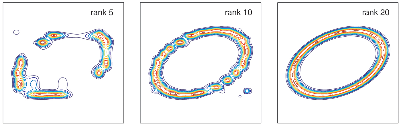
Figure 1. Iterative Gaussian elimination applied to f(x,y) = exp(–100(x2 – xy + 2y2 – 1/2)2) in the unit square, with contour levels at 0.1, 0.3, . . . , 0.9. At rank 88, f is approximated to 16-digit accuracy. This is an analogue for functions of the rounding of real numbers to floating-point numbers.
|
For numerical computing with functions, the key challenge is not just to represent functions, but to compute with them. Every time an operation like \(fg\) or sin\((f)\) is carried out, Chebfun2 constructs an approximation of the result with rank truncated to achieve about 16 digits of accuracy, just as IEEE arithmetic truncates the result of an operation like \(xy\) or sin\((x)\) to 64-bit precision.
In Chebfun2, rounding operations like the one illustrated in Figure 2 happen all the time, whenever a function is operated on or two functions are combined. On this technology we build function evaluation, integration, differentiation, vector calculus, optimization, and other operations. The power is not yet as great as that of one-dimensional Chebfun, which can deal with singularities and solve differential equations, but it is still remarkable. Chebfun2 solves Problem 4 of the 2002 SIAM 100-Digit Challenge [2], involving the global minimization of a complicated function, to 12-digit accuracy in less than a second! Challenges ahead include the extension of these ideas to differential equations, functions with singularities, more general domains, and higher dimensions, and the development of theory to quantify the convergence of these low-rank approximations.
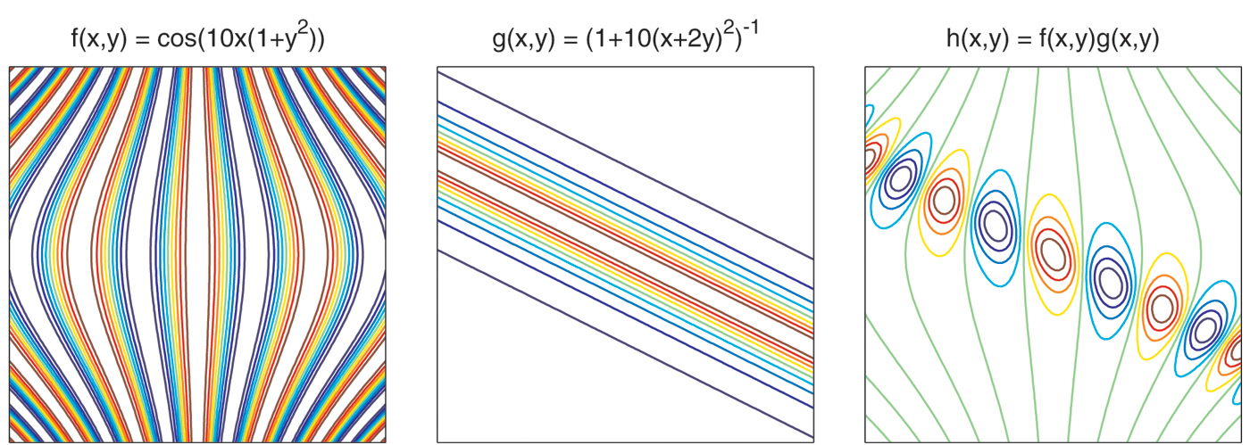
Figure 2. Iterative GE approximates functions f and g over the unit square to 16-digit accuracy by approximants of ranks 19 and 85, respectively. The product h = fg is approximated to the same accuracy with rank 96, not rank 1615 as one would expect mathematically. This is an analogue for functions of the rounding of a product xy in floating-point arithmetic.
|
Gaussian elimination is an iterative algorithm too.
References
[1] M. Bebendorf, Hierarchical Matrices, Springer, New York, 2008.
[2] F. Bornemann et al., The SIAM 100-Digit Challenge: A Study in High-Accuracy Numerical Computing, SIAM, Philadelphia, 2004.
[3] O.A. Carvajal, F.W. Chapman, and K.O. Geddes, Hybrid symbolic-numeric integration in multiple dimensions via tensor-product series, in Proceedings of ISSAC ’05, M. Kauers, ed., ACM Press, New York, 2005, 84–91.
[4] W. Hackbusch, Tensor Spaces and Numerical Tensor Calculus, Springer, New York, 2012.
[5] M.W. Mahoney and P. Drineas, CUR matrix decompositions for improved data analysis, Proc. Natl. Acad. Sci. USA, 106 (2009), 697–702.
[6] A. Townsend, Chebfun2 software, http://www.maths.ox.ac.uk/chebfun, 2013.
[7] A. Townsend and L.N. Trefethen, An extension of Chebfun to two dimensions, SIAM J. Sci. Comput., submitted.[8] E.E. Tyrtyshnikov, Mosaic-skeleton approximations, Calcolo, 33 (1996), 47–57.
Alex Townsend is a graduate student in the Numerical Analysis Group at the University of Oxford, where Nick Trefethen is a professor.