The Dark Side of Image Reconstruction

By Rebecca Willett

Many scientific and engineering applications rely on the accurate reconstruction of spatially, spectrally, and temporally distributed phenomena from photon-limited data. Night vision, with small amounts of light incident upon a camera’s aperture, is a classic example of photon-limited imaging. Photon limitations are also pervasive in fluorescence microscopy. Here, high-quality raw images with large photon counts require (a) long data acquisition times that limit experimental throughput and preclude moving specimens, (b) high laser power that kills living specimens, or (c) large quantities of fluorescent dye that are toxic for living cells. Photon-limited spectral imaging, in which we measure a scene’s luminosity at each spatial location for many narrow spectral bands, plays a critical role in environmental monitoring, astronomy, and emerging medical imaging modalities, such as spectral computed tomography.

When the number of observed photons is very small, accurately extracting knowledge from the data requires the development of both new computational methods and new theory. This article describes (a) a statistical model for photon-limited imaging, (b) ways in which low-dimensional image structure can be leveraged for accurate photon-limited image denoising, and (c) implications for photon-limited imaging system design. 

Problem Formulation

Imagine aiming a camera at a point in space and observing photons arriving from that location. If you could collect photons for an infinite amount of time, you might observe an average of, say, 3.58 photons per second. In any given second, however, you receive a random quantity of photons, say 3 or 10. The number of photons observed in a given second is a random quantity, well modeled by the Poisson distribution. We would like to estimate this average photon arrival rate based on the number of photons collected during a single second for each pixel in a scene. We can model the observed photons over an arbitrary period of \(T\) seconds (cf. [20]):

\[\begin{equation}\tag{1}
y \sim {\mathrm{Poisson}}(TAf^{*})\\
\mathrm{or} \\
y_{i} \sim {\mathrm{Poisson}}~(T \sum_{j} A_{ij}f_{j}^{*}) , 
\end{equation}\]

where \(f^{*} \in \mathbb{R}^{p}_{+}\), with \(|f^{*}|_{1} = 1\), is the true image of interest, with \(p\) pixels; \(A \in  [0, 1]^{­n \times p}\) is an operator corresponding to blur, tomographic projections, compressed sensing measurements, or any other linear distortion of the image, where \(n\) is the number of photon sensors in our imaging system; and \(T \in \mathbb{R}_+\) corresponds to the data acquisition time or overall image intensity.

That is, \(y_i\) is the observed number of photons at detector element \(i\), and \(f^{*}_{j}\)is the average photon arrival rate associated with pixel \(j\) in the scene. Our goal is to estimate \(f^{*}\) from \(y\).

Accurate estimation requires simultaneously leveraging Poisson statistics, accounting for physical constraints, and exploiting low-dimensional spatial structure within the image. 

Image estimation and linear inverse problems have received widespread attention in the literature, but accounting for Poisson noise explicitly, though critical, is not addressed by most methods. Finding and exploiting low-dimensional structure in photon-limited settings present a myriad of unique computational and statistical challenges.

Sparsity and Low-dimensional Structure in Image Denoising

We first consider the special case of \(A = I_{p}\), the identity matrix, and \(n = p\). In this setting, we essentially observe a “noisy” version of the scene of interest and wish to estimate the underlying image, as depicted in Figure 1(a) and (b). This image corresponds to the flag arm patch worn by US armed forces so that they can readily identify each other using night vision cameras.

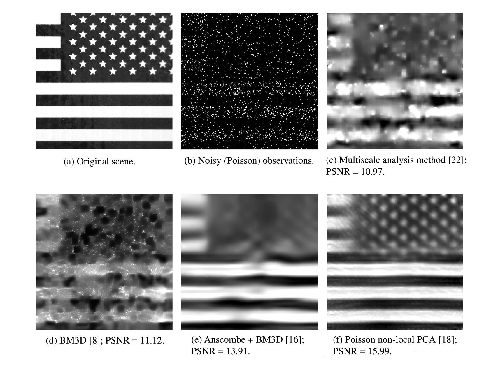
Figure 1. Photon-limited image denoising. The multiscale method in (c) was representative of the state of the art in the early 2000s; since then, methods like BM3D [8], which exploit low-rank structure among the collection of all patches in an image, have emerged at the forefront of image denoising. Simply applying methods like BM3D (which were designed for Gaussian noise) directly to Poisson images yields poor results, as shown in (d). Applying the Anscombe transform to Poisson data generates approximately Gaussian data that can be processed using tools like BM3D, as demonstrated in (e). Methods designed explicitly for Poisson data can reveal additional structure, as shown in (f).

Fifteen years ago, a large community focused on wavelet-based methods for image denoising. Simple wavelet coefficient shrinkage procedures are effective in Gaussian noise settings because the noise in the wavelet coefficients is uncorrelated, identically distributed, and signal-independent. These nice noise properties do not hold in the presence of Poisson noise, so these methods yield estimates with significant artifacts. To address this challenge, many researchers proposed methods designed to account explicitly for Poisson noise [2–5, 14, 15, 19, 21–23]. The result of one of these methods (a state-of-the-art multiscale method, based on a computationally efficient recursive partitioning scheme) is illustrated in Figure 1(c) [22, 23].

Modern denoising methods leverage additional low-dimensional structure within images. For instance, BM3D divides a noisy image into overlapping patches (i.e., blocks of pixels), clusters the patches, stacks all the patches in each cluster to form a three-dimensional array, and applies a three-dimensional transform coefficient shrinkage operator to each stack to denoise the patches [8]. The denoised patches can then be aggregated to form a denoised image. The result of applying BM3D directly to photon-limited image data is shown in Figure 1(d); significant artifacts are present because of the failure to account for the Poisson statistics in the data.

Simply transforming Poisson data to produce data with approximate Gaussian noise via the Anscombe transform [1] can be effective when the photon counts are uniformly high [6, 24]. Specifically, for each pixel we compute the Anscombe transform, \(z_{i} = 2 \sqrt{y_{i} + 3/8}\) for sufficiently large \(y_{i}\), we know that \(z_i\) is approximately Gaussian with unit variance. Hence, we can apply a method like BM3D to the transformed image \(z_i\) and invert the Anscombe transform to estimate \(f^{*}\). Historically, this approach performed poorly at low photon count levels, but recent work on statistically unbiased inverse Anscombe transforms (as opposed to an algebraic inverse Anscombe transform) [16] has resulted in far better estimates, as shown in Figure 1(e).

When photon counts are very low, it is better to avoid the Anscombe transform and tackle Poisson noise directly. For instance, the nonlocal Poisson principal component analysis (PCA) denoising method performs noisy image patch clustering, subspace estimation, and projections for each cluster (similar to the BM3D approach outlined above); within each of these steps, however, the optimization objectives are based on the Poisson log-likelihood and account naturally for the non-uniform noise variance [18]. This approach can yield significant improvement in image quality, as shown in Figure 1(f); further potential improvements have been demonstrated very recently [12].

Photon-limited Problems

So far, we have seen that sparsity and low-dimensional structure can play a critical role in extracting accurate image information from low-photon-count data. We now address a related question:

Given our understanding of the role of sparsity in image denoising, can we design smaller, more efficient, or more accurate imaging systems? 

The preceding section focused on denoising problems, in which \(A\) from (1) was the identity operator. In this section we examine inverse problems, where \(A\) is a more general (known) operator that describes the propagation of light through an imaging system. Computational imaging is focused on the design of systems and associated system matrices \(A\) that will facilitate accurate estimation of \(f^{*}\).

Consider, for instance, the single-pix­­el camera developed at Rice University [9] (Figure 2) and the similar single-pixel fluorescence microscope. The idea is to collect successive single-pixel projections of a scene, based on compressed sensing principles, and then reconstruct the high-resolution scene from a relatively small number of measurements. The digital micromirror device at the heart of this design can operate at very high frequencies, allowing the collection of many measurements in a short time. However, given a fixed time budget for data acquisition (\(T\)), larger numbers of measurements imply less time (and hence fewer photons) per measurement. Is it better, then, to collect a large number of diverse but low-quality, photon-limited measurements, or a smaller number of higher-quality measurements? How quickly can we acquire such compressive data while ensuring our ability to reconstruct the scene?

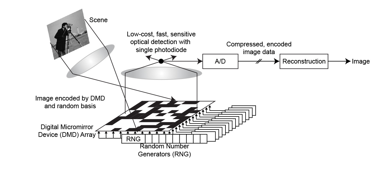
Figure 2. The single-pixel camera developed at Rice [9].

 

Similar questions arise in the context of tomography, as depicted in Figure 3. In applications like pediatric x-ray CT, we operate in photon-limited conditions to ensure patient safety. Given a limited patient dose (which is proportional to the number of photons we can collect and the time budget \(T\)), is full-angle tomography with relatively noisy measurements better or worse than measuring only a small subset of the possible projections with higher fidelity?

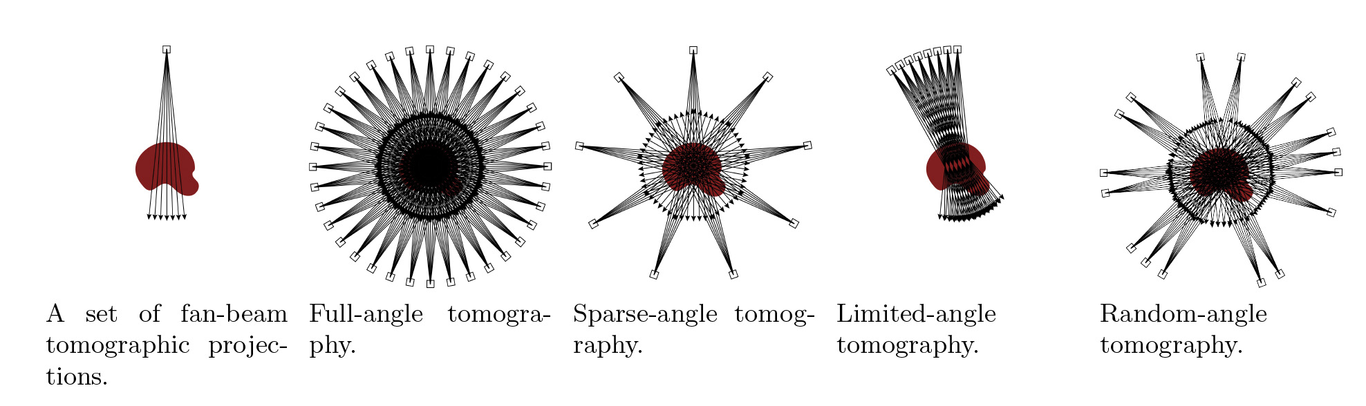
Figure 3. Various tomographic imaging system designs.

Unfortunately, most work on compressed sensing and inverse problems does not address such tradeoffs. To see why, think of the system matrix entry \(A_{ij}\) as corresponding to the probability of a photon from location \(j\) in \(f^{*}\) hitting the detector at location \(i\); this interpretation implies that \(A_{ij} \in [0, 1]\) and that the columns of \(A\) sum to at most 1. Matrices considered in most of the compressed sensing literature (such as those that satisfy the restricted isometry property  (RIP) [25]) do not satisfy these constraints! Rescaling RIP matrices to satisfy physical constraints introduces new performance characterizations and tradeoffs; photon-limited compressed sensing thus differs dramatically from compressed sensing in more conventional settings, as summarized in Table 1 [13].

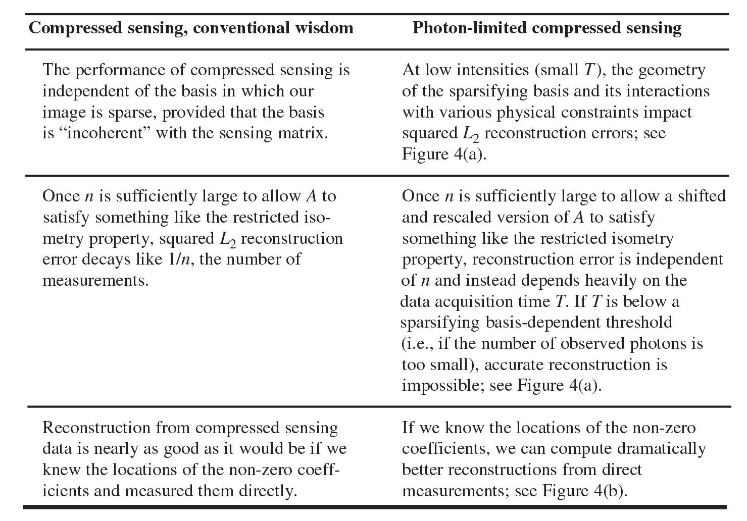
Table 1. Compressed sensing in conventional and photon-limited settings.

 

In particular, the analysis in [6] helps address our earlier question, whether it is better to have many photon-limited measurements or few photon-rich measurements. The number of measurements, \(n\), needs to be large enough to ensure that the sensing matrix \(A\) will facilitate accurate reconstruction, e.g., \(A\) corresponds to a RIP-satisfying matrix that has been shifted and rescaled to reflect the above-mentioned physical constraints. Once this condition is satisfied, \(n\) does not control mean squared error performance––suggesting that many photon-limited measurements and few photon-rich measurements are equally informative, and system designers can choose whatever regime is cheapest, lightest, or easiest to calibrate. We also see that there is a time threshold \(T_{0}\), and if the data acquisition time \(T\) is below \(T_0\), then accurate reconstruction is impossible. Thus, even if hardware advances like faster digital micromirror devices allow us to collect measurements more rapidly, we cannot reduce the total data acquisition time below \(T_0\).

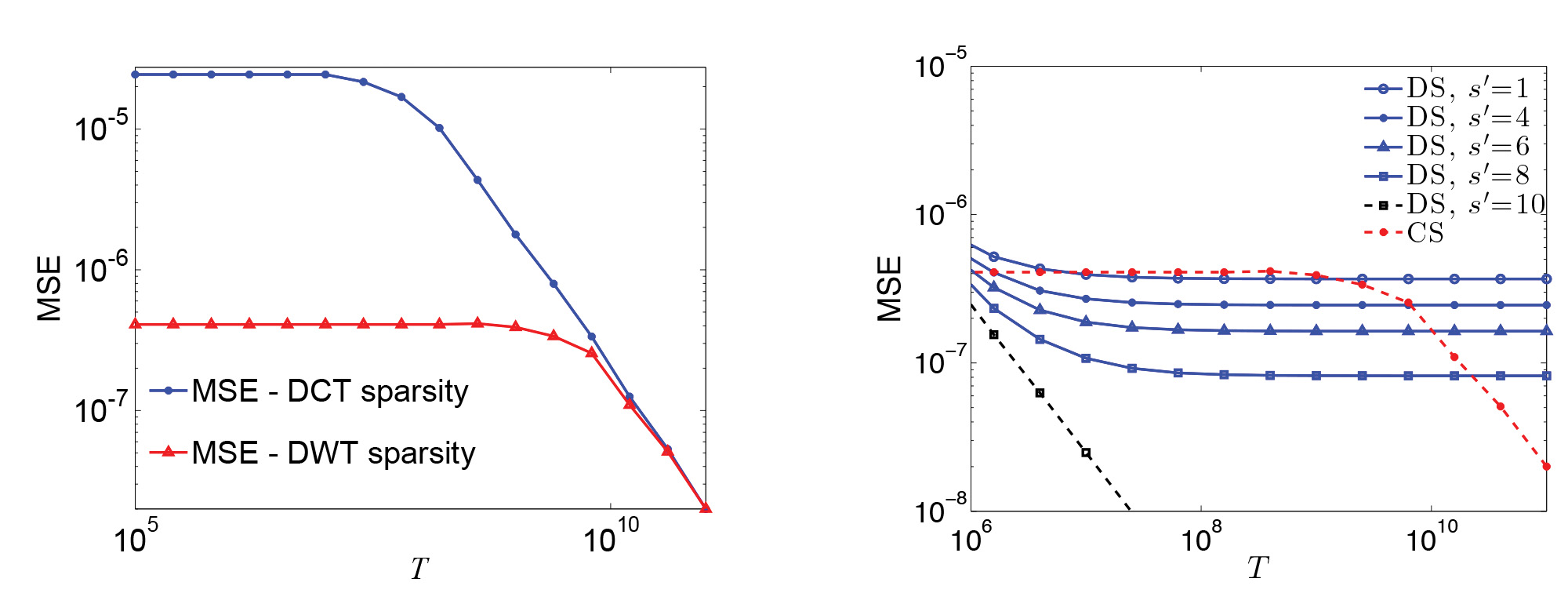
Figure 4. Photon-limited compressed sensing. Left: mean squared error (MSE) as a function of data acquisition time T for two different images, each sparse in a different basis: discrete cosine transform (DCT) and discrete wavelet transform (DWT). For sufficiently large T, the error decays like 1/T, but in low-photon-count regimes we cannot reliably reconstruct the images. The minimum T necessary for reliable reconstruction depends on the choice of sparsifying basis. Right: mean squared error as a function of data acquisition time T for different sampling schemes. The images here are sparse in a wavelet basis, and s’ is the number of coarse-scale non-zero wavelet coefficients. The total number of non-zero coefficients s is 10. DS refers to downsampling---i.e., measuring a low-resolution version of the image directly. CS refers to compressed sampling with a dense random sensing matrix; the curve is the same regardless of s'. We see that downsampling can significantly outperform compressed sensing at low-photon-count levels.

Conclusions

In general, photon-limited image reconstruction methods and optical system designs that fail to account for the statistics and physical constraints of photon-limited imaging will yield results dramatically worse than what we can achieve by accounting for those constraints. Compressed sensing analyses in particular are often based on methods and assumptions that are not compatible with these constraints, and thus sometimes provide bounds that are not achievable in practical settings. Bounds that take these constraints and statistics into account reveal very different behaviors and, ultimately, could contribute to improved optical sensor design strategies. So become seduced by the dark side of imaging––photon limitations introduce novel challenges and exciting opportunities in imaging science!

References
[1] F.J. Anscombe, The transformation of Poisson, binomial and negative-binomial data, Biometrika, 35 (1948), 246–254.
[2] A. Antoniadis and T. Sapatinas, Wavelet shrinkage for natural exponential families with quadratic variance functions, Biometrika, 88:3 (2001), 805–820.
[3] R. Beran and L. Dümbgen, Modulation of estimators and confidence sets, Ann. Statist., 26 (1998), 1826–1856.
[4] P. Besbeas, I. De Feis, and T. Sapatinas, A comparative simulation study of wavelet shrinkage estimators for Poisson counts, Internat. Statist. Rev., 72:2 (2004), 209–237.
[5] A. Bijaoui and G. Jammal, On the distribution of the wavelet coefficient for a Poisson noise, Signal Process., 81 (2001), 1789–1800.
[6] J. Boulanger, C. Kervrann, P. Bouthemy, P. Elbau, J-B. Sibarita, and J. Salamero, Patchbased nonlocal functional for denoising fluorescence microscopy image sequences, IEEE Trans. Med. Imag., 29:2, (2010), 442–454.
[7] E.J. Candès, The restricted isometry property and its implications for compressed sensing, Comptes Rendus–Mathématique, 346:9/10, (2008), 589–592.
[8] K. Dabov, A. Foi, V. Katkovnik, and K. Egiazarian, Image denoising by sparse 3-d transform-domain collaborative filtering, IEEE Trans. Image Process., 16:8 (2007), 2080–2095.
[9] M. Duarte, M. Davenport, D. Takhar, J. Laska, T. Sun, K. Kelly, and R. Baraniuk, Single pixel imaging via compressive sampling, IEEE Signal Processing Mag., 25:2 (2008), 83–91. 
[10] M. Fisz, The limiting distribution of a function of two independent random variables and its statistical application, Colloq. Math., 3 (1955), 138–146.
[11] P. Fryźlewicz and G. P. Nason, Poisson intensity estimation using wavelets and the Fisz transformation, Tech. Rep., Department of Mathematics, University of Bristol, United Kingdom, 2001.
[12] R. Giryes and M. Elad, Sparsity based Poisson denoising with dictionary learning, 2013; arXiv:1309.4306.
[13] X. Jiang, G. Raskutti, and R. Willett, Minimax optimal rates for Poisson inverse problems with physical constraints, submitted, 2014; arXiv:1403:6532. 
[14] E. Kolaczyk, Bayesian multi-scale models for Poisson processes, J. Amer. Statist. Assoc., 94 (1999), 920–933.
[15] E. Kolaczyk and R. Nowak, Multiscale likelihood analysis and complexity penalized estimation, Ann. Statist., 32 (2004), 500–527.
[16] M. Mäkitalo and A. Foi,  Optimal inversion of the Anscombe transformation in low-count Poisson image denoising, IEEE Trans. Image Process., 20:1 (2011), 99–109.
[17] M. Mäkitalo and A. Foi, Optimal inversion of the generalized anscombe transformation for Poisson–Gaussian noise, submitted, 2012. 
[18] J. Salmon, Z. Harmany, C. Deledalle, and R. Willett, Poisson noise reduction with non-local PCA, J. Math. Imaging Vision, 48:2 (2014), 279–294; arXiv:1206:0338.
[19] S. Sardy, A. Antoniadis, and P. Tseng, Automatic smoothing with wavelets for a wide class of distributions, J. Comput. Graph. Statist., 13:2 (2004), 399–421.
[20] D. Snyder, Random point processes, Wiley-Interscience, New York, 1975.
[21] K. Timmermann and R. Nowak, Multiscale modeling and estimation of Poisson processes with application to photon-limited imaging, IEEE Trans. Inform. Theory, 45:3 (1999), 846–862.
[22] R. Willett and R. Nowak, Multiscale Poisson intensity and density estimation, IEEE Trans. Inform. Theory, 53:9 (2007), 3171–3187; doi:10.1109/TIT.2007.903139.
[23] R. Willett and R. Nowak, Platelets: A multiscale approach for recovering edges and surfaces in photon-limited medical imaging, IEEE Trans. Med. Imaging, 22:3 (2003), 332–350; doi:10.1109/TMI.2003.809622.
[24] B. Zhang, J. Fadili, and J.-L. Starck, Wavelets, ridgelets, and curvelets for Poisson noise removal, IEEE Trans. Image Process., 17:7 (2008), 1093–1108.

Rebecca Willett is an associate professor in the Department of Electrical and Computer Engineering at the University of Wisconsin-Madison. This article is based on her invited talk at the 2014 SIAM Conference on Imaging Sciences.