Accurate Mathematical Modeling of Wind Turbines Improves Their Implementation

By Sameh A. Eisa

Figure 1. Wind turbine (WT) power system. WT dynamics act as a system with internal dynamics (such as mechanical, electrical, and control parts) that both interact with and are affected by external parameters and profiles, which are unpredictable and have their own uncontrollable conditions (like wind speed and power grid load). Figure courtesy of Sameh Eisa.

Governments and corporations alike seek to understand the challenges and consequences of integrating wind turbines (WTs) with both other power systems and the power grid. Said integration is complex and challenging, as WT power systems are very different from traditional systems; they experience inherent fluctuations and have less predictability, less stabilizing inertia for the grid, and more sensitivity to uncontrollable conditions like weather. Research in control systems, optimization, power generation, and energy storage has increased dramatically over the last decade in response to the complexity of WT implementation. However, unintended consequences that can negatively affect the entire power grid remain a major concern [7].

WT modeling is a major focus in both academia and industry, as accurate models of WT power systems enable more sophisticated study, design, simulation, and experimentation and extend the potential for efficient data-driven approaches. The industry’s modeling frameworks—such as that of General Electric (GE) [1]—have mainly concentrated on S-domain/frequency-domain formulation and modeling. Corporations argue that this approach is sufficient for their targeted studies, which often address local stability and control methods in a particular situation or condition. However, we determined that an accurate, well-posed, time-domain mathematical model of WT power systems is crucial if scientists hope to deeply understand the dynamics of WTs and the consequences of large-scale integration within the power grid. 

Figure 2. Measured real data from a wind turbine (blue stars) compared to power-wind speed curves from our model in [3, 4] (solid red line) and the model in [8, 9] (dashed red line). Figure courtesy of Sameh Eisa.

We converted the modeling foundations and industrial specifications from industrial and technical reports by GE and other organizations into a nonlinear, time-domain system of differential-algebraic equations that is mathematically well-posed [6]. The resulting system enables a wide range of analysis and simulation. More information about the mathematical modeling of WT power systems (see Figure 1) and the outcome of accurate mathematical time-domain analysis and simulations is available in [3, 4].

We formulate our WT power system as a differential-algebraic equation system in the following semi-explicit form [3, 4]:

\[\boldsymbol{\dot x} = \boldsymbol{f}(t, \boldsymbol{p}, \boldsymbol{x}, \boldsymbol{y}), \quad \boldsymbol{x}(t_0) = \boldsymbol{c},\tag1\]

\[\mathbf{0} = \boldsymbol{g}(t, \boldsymbol{p}, \boldsymbol{x}, \boldsymbol{y}).\]

Here, \(\boldsymbol{x}\) represents the differential state variables, \(\boldsymbol{y}\) represents the algebraic state variables, \(\boldsymbol{p}\) represents the system’s parameters, and \(\boldsymbol{c}\) represents the initial conditions of the differential state variables. The states \(\boldsymbol{x}\) include physical variables such as angular velocities (turbine and generator speeds), while the states \(\boldsymbol{y}\) involve variables from the connection to the power grid, like the terminal voltage. The parameters \(\boldsymbol{p}\) are critical for the WT power system because they describe many time-invariant and time-varying cases/profiles, including uncontrolled input, stochastic input, design-fixed-valued input, and a generated control signal. We validate our model of the form \((1)\) against measured data and compare it to other S-domain/frequency-domain models from the literature (see Figure 2).

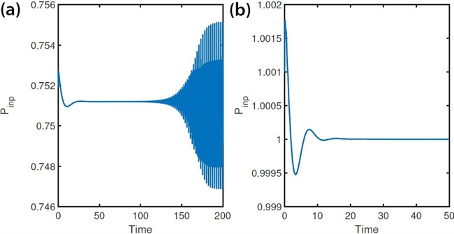
Figure 3. The state of (input) electric power in a wind turbine (WT) power system that is simulated under a particular load in the power grid (suddenly changed, then cleared). 3a. Simulation with medium wind speed. 3b. Simulation with high wind speed. The power will continuously oscillate in this simulation case when wind speed is in a medium range (note that we tested cases when oscillations also occur in high wind speeds), manifesting a Hopf bifurication. Meanwhile, the control limiters alternately tolerate and prevent this phenomenon. When power that oscillates in this way is delivered to the power grid, the grid’s stabilizing inertia is weakened. This effect represents a vulnerability in the system’s resilience, since uncontrollable changes in the grid lead to problematic behavior in the WT that is reflected back into the grid. The National Renewable Energy Laboratory has observed this occurrence, and our mathematical model used theory and simulation to capture and explain it [5]. Figure courtesy of Sameh Eisa.

Here, we briefly provide some results from the rigorous and time-domain mathematical modeling of WT power systems:

1. WT power systems are highly sensitive and possibly unstable due to external parameters and profiles, such as wind speed \(v_\textrm{wind}\) and power grid loads (resistance \(\textrm{R}\) and reactance \(\textrm{X}\) loads).
2. When using the typical pitch and torque controls from industry, WT power systems are under-actuated (i.e., the number of controls is less than the number of states of interest) with respect to many desired outputs.
3. WT power systems are not safe with the control limiters that industry suggests because they are unable to stop the effects of many sudden changes and faults. As a result, the system’s states—including heavy mechanical parts—can become unstable or continuously oscillating (see Figure 3).
4. WT power systems are usually stabilizable to an extent in extreme situations if one applies a user-defined signal called Q droop (introduced by GE) to the reactive power portion of the system.

We believe that rigorous time-domain mathematical modeling has unequivocally advanced our understanding and analysis of WT systems and will ultimately improve system resilience and make renewables a more reliable source of energy. The mathematical modeling of wind turbine systems is indispensable, and other emerging green technologies must follow suit.

References
[1] Clark, K., Miller, N.W., & Sanchez-Gasca, J.J. (2010). Modeling of GE wind turbine-generators for grid studies. Schenectady, NY: General Electric International, Inc.. Retrieved from https://www.researchgate.net/publication/267218696_Modeling_of_GE_Wind_Turbine-Generators_for_Grid_Studies_Prepared_by. 
[2] Department of Energy. (2021, August 30). DOE releases new reports highlighting record growth, declining costs of wind power. Retrieved from https://www.energy.gov/articles/doe-releases-new-reports-highlighting-record-growth-declining-costs-wind-power.
[3] Eisa, S.A. (2019). Modeling dynamics and control of type-3 DFIG wind turbines: Stability, Q droop function, control limits and extreme scenarios simulation. Electr. Power Syst. Res., 166, 29-42.
[4] Eisa, S.A. (2019). Nonlinear modeling, analysis and simulation of wind turbine control system with and without pitch control as in industry. In R.-E. Precup, T. Kamal, & S.Z. Hassan (Eds.), Advanced control and optimization paradigms for wind energy systems (pp. 1-40). Singapore: Springer.
[5] Eisa, S.A. (2020). Investigating the problem of oscillatory orbits and attractors in wind turbines system under control limits imposed by industry. Electr. Power Syst. Res., 180, 106098.
[6] Eisa, S.A., Stone, W., & Wedeward, K. (2017). Mathematical analysis of wind turbines dynamics under control limits: Boundedness, existence, uniqueness, and multi time scale simulations. Int. J. Dynam. Cont., 6, 929-949.
[7] Liang, X. (2016). Emerging power quality challenges due to integration of renewable energy sources. IEEE Trans. Ind. Appl., 53(2), 855-866.
[8] Pourbeik, P, Akhmatov, V., Akiyama, Y., Beaulieu, D., Boyer, R., Ebrahimian R., … Kazachkov, Y. (2007). Modeling and dynamic behavior of wind generation as it relates to power system control and dynamic performance (CIGRE Technical Brochure 328). Paris, France: International Council on Large Electric Systems.
[9] Tsourakis, G., Nomikos, B.M., & Vournas, C.D. (2009). Effect of wind parks with doubly fed asynchronous generators on small-signal stability. Electr. Power Syst. Res., 79(1), 190-200.

Sameh A. Eisa is an assistant professor of aerospace engineering and engineering mechanics at the University of Cincinnati, where he is also the principle investigator of the Modeling, Dynamics, and Control Lab. His interdisciplinary background and current research combine the mathematical and engineering sciences. Eisa holds a B.Sc. in electrical engineering and a Ph.D. in applied and industrial mathematics. He is interested in nonlinear dynamics, control theory, and their applications in bio-inspired systems and renewable energy.