The Race to Compute High-order Gauss–Legendre Quadrature

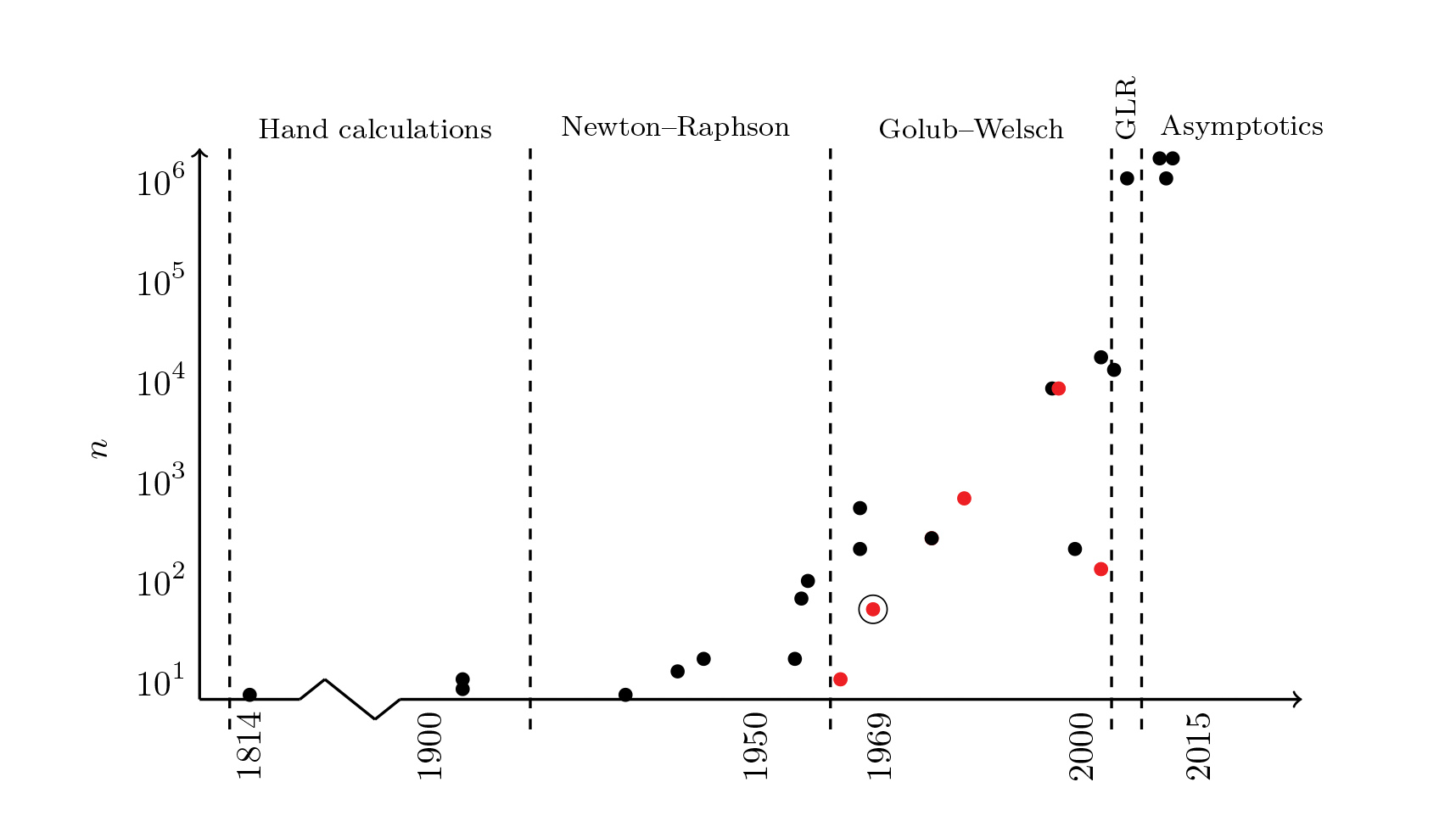
Figure 1. The 100-year race for high-order Gauss–Legendre quadrature. A dot represents published work, located by the publication year and the largest Gauss–Legendre rule reported therein. A red dot indicates a paper based on variants of the Golub–Welsch algorithm. The dot for Golub and Welsch (1969) is circled. For a list of the papers used, click here.

Hand calculations led the way for over a century. Tallquist (1905), Moors (1905), Nyström (1930), and Bayly (1938) used fountain pens and dogged determination to calculate the quadrature nodes for \(n ≤ 12\). Eventually, presumably with a small army of human calculators, Lowan, Davids, and Levenson (1942) tabulated the nodes and weights for \(1 ≤ n ≤ 16\) for the Mathematical Tables Project.

A decade later computers were beginning to dominate tedious hand calculations, and large tabulations of nodes and weights were profitably published. The most popular algorithm for computing Gauss nodes was the Newton–Raphson method for finding the roots of \(P_n(x)\) with a three-term recurrence used to evaluate \(P_n\) and \(P^{'}_n\) . Huge strides were made. Gawlik (1958) briefly led with \(n = 64\) before Davis and Rabinowitz (1958) got \(n = 96\), and finally Stroud and Secrest (1966) achieved \(n = 512\). This was the golden age for Gauss–Legendre quadrature.

By the 1960s orthogonal algorithms for eigenproblems were hot off the press and Gene Golub was becoming famous. The Golub–Welsch algorithm [5]—featuring both QR and Golub––was momentous. It quickly overshadowed the earlier (1963) result of Rutishauser. Contrary to popular belief, however, the Golub–Welsch algorithm is not, and never was, the state-of-the-art algorithm for computing Gauss–Legendre quadrature rules in terms of accuracy and speed. Yet, by elegantly bringing together eigenproblems and Gauss quadrature, it radically changed how the world computed integrals. Before 1969, a few would compute quadratures by carefully extracting the tabulated values from Stroud and Secrest (1966) and calculating (1). After 1969, all were computing Gauss nodes and weights for themselves. Tabulations were already falling out of favor across the computational sciences; the Golub–Welsch algorithm made it so for Gauss nodes and weights as well. This makes 1969 a year to remember for more than just the moon landing.

In the years that followed, only a handful of experts noticed improvements to the details of the Newton–Raphson approach produced by Lether (1978), Yakimiw (1996), Petras (1999), and Swarztrauber (2003). While the Golub–Welsch algorithm was computing a few hundred nodes and weights, the Newton–Raphson approach was computing thousands. Many, still unaware of the developments after 1969, have concluded that Gauss–Legendre quadrature is not computationally feasible for large \(n\). Attention has shifted to adaptive and piecewise quadrature schemes.

In 2007 Glaser, Lui, and Rokhlin described a ground-breaking algorithm that can compute a million quadrature nodes in a handful of seconds [4]. Accolades should have followed, but the algorithm failed to awaken much interest. A few years later Bogaert, Michiels, and Fostier [2] and Hale and Townsend [6] showed that the Newton–Raphson method for finding the roots of \(P_n(x)\) with careful evaluation of \(P_n\) and \(­P_{n}^{'}\) by asymptotic formulas could be just as fast and more accurate than anything the world had seen before.* The golden age had returned. Figure 2 shows the quadrature error (see equad in [6] for the exact definition) and the timings for five historically important algorithms. It was after careful numerical comparisons like these that the race was fully appreciated. 

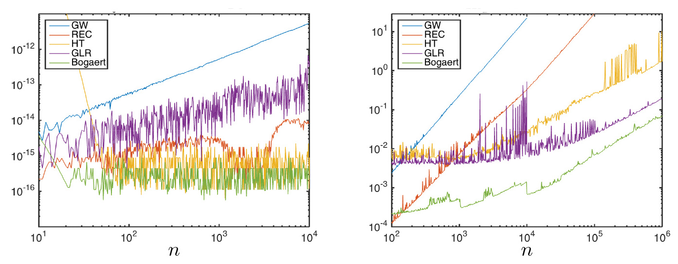
Figure 2. Quadrature error (left) and computational time (right) for Gauss–Legendre nodes and weights computed by the Golub–Welsch algorithm [5] (GW), Newton–Raphson with three-term recurrence (REC), Newton–Raphson with asymptotic formulas [6] (HT), the Glaser–Lui–Rokhlin algorithm [4] (GLR), and Bogaert's formulas [1] (Bogaert). The timings given here are for implementations in different programming languages and cannot be used for direct comparisons.

The epilogue was written by Bogaert a few months ago [1]. He derived explicit asymptotic formulas for the Gauss–Legendre nodes and weights that are accurate to 16 digits for any \(n ≥ 20\). Using his formulas, I just computed one billion and two Gauss–Legendre nodes and weights on my laptop. This is a world record! So large is this rule that nodes that are near neighbors of ±1 are identical to 15 decimal places. It now takes less than a millisecond to compute a thousand nodes and less than a tenth of a second to compute a million.  

Ignace Bogaert is the winner of the 100-year race. Bravo! 

It was a fun race with a deserving winner. We are now searching for applications that require thousands of nodes and weights. Our algorithms are poised for use. If you have an application in mind, please email [email protected]. 

One million Gauss–Legendre nodes and weights––no problem. But how will we use them?

*See [6] for computing Gauss–Jacobi, Gauss–Lobotto, and Gauss–Radau quadratures.

Acknowledgments: I thank Ignace Bogaert and Nick Hale for helpful comments and suggestions, and Nick Trefethen for encouraging me to write this article.

References

[1] I. Bogaert, Iteration-free computation of Gauss–Legendre quadrature nodes and weights, SIAM J. Sci. Comput., 36 (2014), C1008–C1026.
[2] I. Bogaert, B. Michiels, and J. Fostier, \(\mathcal{O}(1)\) computation of Legendre polynomials and Gauss–Legendre nodes and weights for parallel computing, SIAM J. Sci. Comput., 34 (2012), C83–C101.
[3] C.F. Gauss, Methodus nova integralium valores per approximationem inveniendi, Comment. Soc. Reg. Scient. Gotting. Recent., (1814), 39–76.
[4] A. Glaser, X. Liu, and V. Rokhlin, A fast algorithm for the calculation of the roots of special functions, SIAM J. Sci. Comput., 29 (2007), 1420–1438.
[5] G.H. Golub and J.H. Welsch, Calculation of Gauss quadrature rules, Math. Comp., 23 (1969), 221–230.
[6] N. Hale and A. Townsend, Fast and accurate computation of Gauss–Legendre and Gauss–Jacobi quadrature nodes and weights, SIAM J. Sci. Comput., 35 (2013), A652–A674.
Alex Townsend is an Applied Mathematics Instructor at the Massachusetts Institute of Technology.