By Jorge Nocedal
Optimization is one of the pillars of statistical learning. It plays a crucial role in the design of “intelligent” systems, such as search engines, recommender systems, and speech and image recognition software. These systems, which embody the latest advances in machine learning, have made our lives easier. Their success has created a demand for new optimization algorithms that, in addition to being scalable and parallelizable, are good learning algorithms. Future advances, such as effective image recognition, will continue to rely heavily on methods from statistics and optimization.
It was not supposed to be that way. I remember being dazzled by the promise of artificial intelligence depicted so brilliantly in the 1968 movie 2001: A Space Odyssey. HAL, the personal assistant, had human-like intelligence and even personality. Forty-five years later, that promise has not been realized. Very few people would consider Siri a real personal assistant. Instead of using classical artificial intelligence techniques, the intelligent systems mentioned above rely heavily on statistical learning algorithms. Combined with powerful computing platforms, very large datasets, and expert feature selection, the algorithms form the bases for innovative learning systems that are accessible to the public through “the cloud.” Improvements continue at a rapid rate.
To give an example, in the last few years, deep neural networks have revolutionized speech recognition. Table 1 shows the word error rate for three standard speech recognition tasks, as reported by three leading research centers. The results obtained with deep neural nets are compared with those from earlier systems based on Gaussian mixture models. Although the reduction in error rate with DNN may not seem surprising to an outsider, it is greater than the advances made in the preceding 10 years.
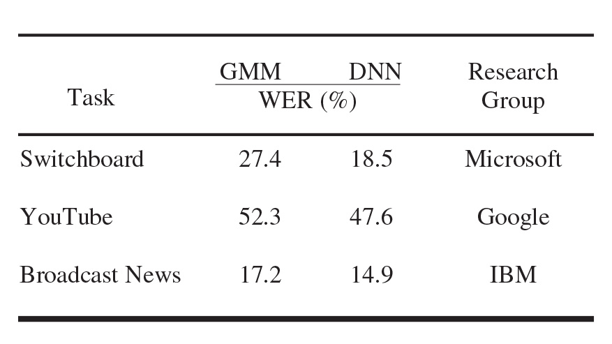
Table 1. Word error rate (WER) for three speech recognition tasks. GMM, Gaussian mixture models. DNN, deep neural nets. Data provided by Brian Kingsbury from IBM. |
Deep neural networks are highly nonlinear, and optimizing their parameters represents a formidable problem. A typical neural network for speech recognition has between five and seven hidden layers, with about 1000 units per layer, and tens of millions of parameters to be optimized. (See Figure 1.) Training requires up to 1000 hours of speech data, representing on the order of 100 million training examples. Optimizing (i.e., training) a neural network of this size takes two weeks on a supercomputer.
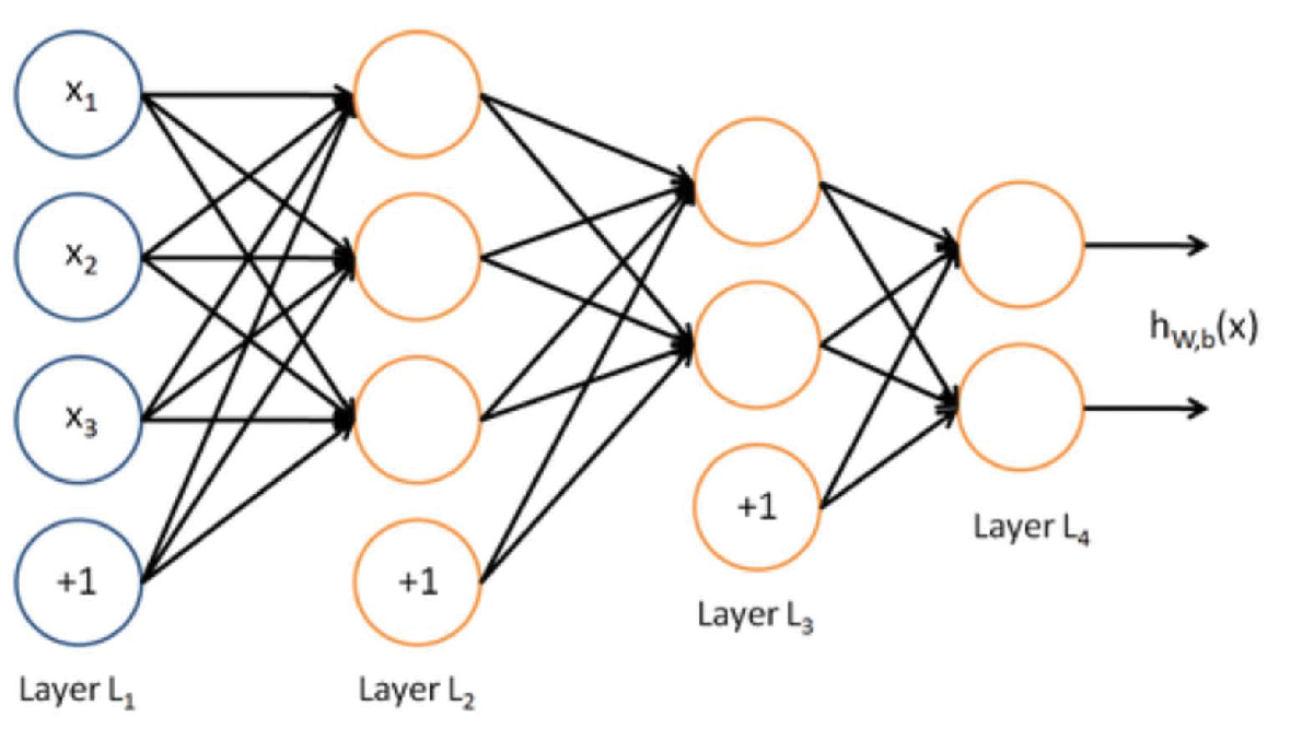
Figure 1. A neural network for speech recognition. |
The new challenge that arises for optimization methods in the machine learning setting, as mentioned earlier, is that they must be good learning algorithms. By this I mean that the hypothesis functions they define must make good predictions on unseen data; it is not enough that the optimization methods perform efficiently on a particular training set. The new demands imposed on optimization algorithms in the context of machine learning––large scale, stochasticity, nonlinearity, parallelism, good generalization––have led to a burst of research activity.
Supervised Learning
This research is best described in the context of supervised learning. We are given a training set of size \(N\); each training point \((x_{i}, z_{i})\) consists of feature information \(x_i\) (think of an acoustic frame 70 milliseconds long) and a correct label \(z_i\) (the word or phoneme) associated with it. We define a prediction function \(h\) that depends on a parameter \(w\), e.g.,
\begin{equation}\tag{1} h(w;x) = w^{T}x \end{equation}
that makes good predictions on unseen data, \(\hat{x}\), i.e.,
\begin{equation}\tag{2}
\hat{z} = w^{T}\hat{x} ~\textrm{and}~ \hat{z} \approx z,
~~~ \textrm{with}~ z ~\textrm{being the correct label}.
\end{equation}
(The prediction function \(h\) could be more complex, as is the case with neural networks.) We also require a loss function \(\ell\) that measures the deviation between a prediction and the data; it could be defined as the square loss, a hinge loss, or a logistic function.
The objective function in supervised learning is typically the sum of error terms, each corresponding to a training point \((x_{i}, z_{i})\):
\begin{equation}\tag{3}
F(w) = \frac{1}{N} \sum\limits_{i=1}^{N} \ell (h(w;x_{i}),z_{i}).
\end{equation}
The goal of the optimization method is to minimize this function, with respect to the model parameters \(w\).
Stochastic vs. Batch Methods In Machine Learning
Optimization methods for machine learning fall into two broad categories: stochastic and batch. A prototypical batch method first chooses a sufficiently large sample of training examples to define (3), and minimizes \(F\) using a standard gradient-based method. The iteration has the familiar form \(w_{k+1} = w_{k} – \alpha_{k}\nabla(w_{k})\), where \(\alpha_{k}\) is a step-length parameter. Although this method is convenient in that it can make use of many established optimization methods, the majority opinion is that it is not the best learning algorithm.
The method of choice in most large-scale machine learning applications is the stochastic gradient method proposed by Robbins and Monro in 1951. A typical implementation chooses a single training point \((x_{j}, z_{j})\) at random, and updates the parameters of the model through the iteration
\begin{equation}\tag{4} w_{k+1} = w_{k} – \alpha_{k}\nabla \ell(h(w_{k} ; x_{j}), z_{j}). \end{equation} In other words, the method acts as if only one training point is revealed at a time. This is not a descent method (the update can easily yield an increase in the objective \(F\)); rather, it is a Markov chain method, and \(w_{k}\) is a random variable. Because the gradient estimate is poor (it is correct only in expectation), the step length \(\alpha_k\) must satisfy \(\alpha_{k} \rightarrow 0\). Under normal conditions, one can show convergence in expectation,
\begin{equation}\tag{5}
|\mathbb{E}[F(w_{k})]-F(w^{*})| \leq C/k,
\textrm{for some constant}~C > 0,
\end{equation}
where \(F(w^{*})\) is the optimal value of (3).
This sublinear rate of convergence can be shown to be optimal for iterations that employ only first-order information in this manner. Now, this optimal rate \(O (1/k)\) is achieved also for testing cost (i.e., for generalization error) as long as each data point is seen only once. Other optimization algorithms do not enjoy this property: A given rate of convergence for training cost does not translate into the same rate for testing cost.
In addition, Bottou and Bousquet [1] argue persuasively that when estimation and optimization error are taken into account, the stochastic gradient method has better work complexity bounds than the batch gradient method. By work complexity we mean the total amount of computational effort to reach a given level of accuracy. These arguments, together with ample computational experience, seem to settle the question in favor of the stochastic gradient method, and might suggest that there is little room for improving the optimization process.
“Semi-stochastic” Methods
The question is far from settled, however. The arguments given above assume a sequential computational setting, but everything changes in a parallel setting. The stochastic gradient method is particularly difficult to parallelize [7], whereas batch methods are not. Moreover, the complexity analysis does not consider newly developed methods that, neither purely stochastic nor purely batch, are sometimes called semi-stochastic.
One method of this type gradually increases the size of the sample \(S_k\) used to define the gradient estimate in iteration (4), which is now given by
\begin{equation}\tag{6}
w_{k+1} =
w_{k} – \alpha_{k} \frac{1}{|S_{k}|} \sum\limits_{i \in S_{k}} \nabla \ell (h(w_{k} ; x_{i}), z_{i}). \end{equation} These methods emulate the stochastic gradient method at the start, but evolve toward the batch regime. It has been shown that this approach enjoys work complexity at least as good as that of the stochastic gradient method [3,6] provided that \(|S_{k}|\) increases geometrically with \(k\).
A semi-stochastic method of a different type achieves variance reduction by computing the full batch gradient periodically, and then updating it gradually [4]. At the beginning of a cycle where the current estimate of the solution is \(\tilde{w}\) the algorithm computes \(\nabla F(\tilde{w})\). Then, for the next m iterations an integer \(j \in \{1, \ldots N\}\) is chosen at random and this vector is updated as
\begin{equation}
v_{k} = \nabla \ell(h(w_{k} ; x_{j}), z_{j})
– \nabla \ell(h(\tilde{w} ; x_{j}), z_{j}) + \nabla F(\tilde{w});
\end{equation}
\(v_k\) is used in lieu of the gradient in the iteration (4).
The last line of research I would like to highlight (and there are several more!) focuses on the design of stochastic and batch methods that emulate Newton’s method. Contrary to the conventional wisdom in the machine learning community that only first-order optimization methods are practical in large-scale learning, methods that incorporate Hessian information in a judicious manner can be quite effective. A batch approach that has proved successful for both logistic regression and neural nets is a matrix-free Newton-CG [2,5], where the Hessian is sub-sampled, i.e., formed using only a small percentage (say, 0.01%) of the sample points appearing in (3). And very recently, a fully stochastic quasi-Newton method has been developed, motivated by the fact that the constant C in (5) depends on the square of the condition number of the Hessian. The quasi-Newton approach is designed to diminish this harmful effect of the condition number on the convergence rate.
It is too early to tell which of these new optimization methods will become established techniques in machine learning. The interested reader can follow this research in, for example, SIAM Journal on Optimization and the proceedings of both the Neural Information Processing Systems conferences and the International Conference on Machine Learning.
References
[1] L. Bottou and O. Bousquet, The trade-offs of large scale learning, Adv. Neural Inf. Process. Syst., 20 (2008), 161–168.
[2] R.H. Byrd, G.M. Chin, W. Neveitt, and J. Nocedal, On the use of stochastic Hessian information in unconstrained optimization, SIAM J. Optim., 21:3 (2011), 977–995.
[3] R.H. Byrd, G.M. Chin, J. Nocedal, and Y.Wu, Sample size selection in optimization methods for machine learning, Math. Prog., 134:1 (2012), 127–155.
[4] R. Johnson and T. Zhang, Accelerating stochastic gradient descent using predictive variance reduction, Adv. Neural Inf. Process. Syst., 26 (2013), 315–323.
[5] J. Martens and I. Sutskever, Learning recurrent neural networks with Hessian-free optimization, Proceedings of the 28th International Conference on Machine Learning, ICML, 2011, 1033–1040.
[6] R. Pasupathy, P.W. Glynn, S. Ghosh, and F. Hahemi, How much to sample in simulation-based stochastic recursions? in review.
[7] B. Recht, C. Re, S. Wright, and F. Niu, Hogwild: A lock-free approach to parallelizing stochastic gradient descent, Adv. Neural Inf. Process. Syst., 24 (2011), 693–701.
Jorge Nocedal is a professor in the department of industrial engineering and management sciences at Northwestern University.