"Bike Tracks," Quasi-magnetic Forces, and the Schrödinger Equation

By Mark Levi

In an invited talk at the 2013 SIAM Conference on Applications of Dynamical Systems, Mark Levi described a recently discovered connection between two distinct objects—the stationary Schrödinger equation and “bicycle tracks.” A request from SIAM News for an article based on the talk elicited the following well-illustrated article.

The stationary Schrödinger equation

\[\begin{equation}{\ddot{x}}+p(t)x=0,\end{equation}\tag{1}\]

where \({p}\) is the given potential, arises in many branches of mathematics, physics, and engineering and has been studied for well over a century. Known also as Hill’s equation, it comes up in studies of the spectrum of the hydrogen atom, in celestial mechanics, particle accelerators, forced vibrations, wave propagation, and many other problems. Hill’s equation plays a central role in explaining the complete integrability of the Korteweg–de Vries equation: One of the most remarkable mathematical discoveries of the last century is that the eigenvalues of the Schrödinger operator remain fixed if the potential \({p}\) evolves according to the KdV equation.

The 1989 Nobel Prize in Physics was awarded to W. Paul for his invention of the Paul trap—an electromagnetic trap that suspends charged particles. The mathematical substance of Paul’s discovery amounts to an observation on Hill’s equation, as Paul explained in his Nobel lecture [10]. (As an alternative to Paul’s computational explanation, a geometrical explanation of the workings of the Paul trap can be found in [5].) The stability of Kapitsa’s famous inverted pendulum (demonstrated experimentally by Stephenson in 1908, about half a century before Kapitsa’s paper) is also explained by the properties of Hill’s equation. Incidentally, a topological explanation of this counterintuitive effect can be found in [6].

The long history of Hill’s equation is reflected in the rich classical literature of the 18th and 19th centuries on the eigenfunctions of special second-order equations (including polynomials of Lagrange, Laguerre, Chebyshev, and Airy’s function), as well as in more recent work on inverse scattering and on the geometry of “Arnold tongues” [1,2,9,11].

Introducing bike tracks, the second partner in the new relationship, Figure 1 shows an idealized bike—a segment \({RF}\) of constant length that can move in the plane as follows: The front \({F}\) is free to move along any path, while the velocity of the rear end \({R}\) is constrained to the direction \({RF}\)—that is, the rear wheel doesn’t sideslip. Figure 2 shows some examples.

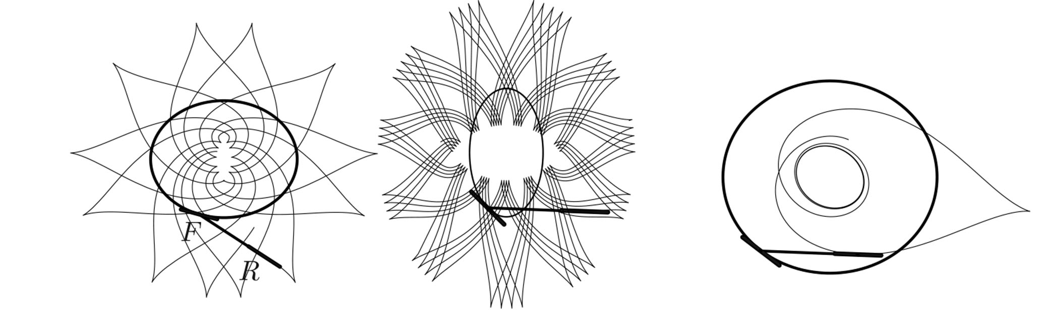
Figure 2. Some paths of the rear wheel as the front wheel traces out the heavier path multiple times. 

The tire track problem does not have the pedigree of the Schrödinger equation, nor does it have the same rich history. Still, the problem has been studied since at least the 1870s (see [3] and references therein). It arises in differential geometry, and also as a model problem in engineering applications; a brief review and further discussion can be found in [4]. (Amusingly, the bicycle can be used to measure areas enclosed by planar curves: The actual device, the Prytz planimeter, is named after its inventor Holger Prytz, a 19th-century Danish cavalry officer.) A beautiful observation of R. Foote [3] gave rise to further developments, including a solution of Menzin’s conjecture from 1908 [8].

To describe the connection between the Schrödinger equation and the tire track problem, I specify a recipe that assigns, to every Schrödinger potential \(p(t)\), the path \((X(t), Y(t))\) of the front wheel in such a way that the Schrödinger equation and the “bicycle equation” are equivalent via an explicit transformation, as explained below.

To understand how the Schrödinger potential \(p\) generates the front wheel path, consider a particle of mass \(m = 1\) whose speed \(\upsilon\) is a prescribed function of time, and whose direction of motion is determined by the force

\[\begin{equation}
{F_N} = {a_N} = \upsilon(2 − \upsilon)
\end{equation}\tag{2}\]

acting in the direction normal to the velocity vector (see Figure 3). Unlike the true magnetic force, this magnetic-like force is not linear in \(\upsilon\). We can think of our particle as a rocket with the “thrust” force acting tangentially to the path, and with the normal “magnetic” force (2) determined by \(\upsilon\). Given \(\upsilon = \upsilon(t)\), the law (2) determines the path \((X(t), Y(t))\) of the particle completely, provided that we fix the initial point and the initial direction. As an example, if we hold \(\upsilon\) constant, we get uniform circular motion, except in the case of \(\upsilon\) = 0 or 1, when uniform rectilinear motion results. Figure 4 shows trajectories for \(\upsilon=\alpha + \beta/(1+{t^2)}\)  and \(\upsilon = \alpha + \beta~cos~t\). Trajectories for \(\upsilon\) of the form \(\upsilon = \alpha + \beta~cos~t + \gamma~cos~2t\) with various choices of \(\alpha\), \(\beta\), \(\gamma\) are shown in Figure 5.

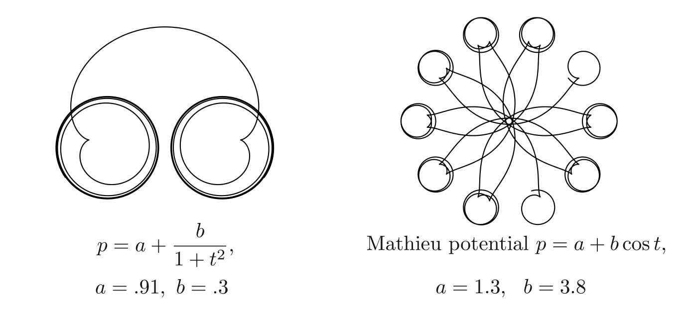
Figure 4. Paths of a particle subject to the strange quasi-magnetic force for various choices of speed \(\upsilon = \upsilon(t)\). Each of these paths corresponds to a Schrödinger potential \(p = p(t) = 1 - \upsilon(t)\).

Given a Schrödinger potential\({p = p(t)}\), we define \(\upsilon = \upsilon(t) = 1 - p\). With \(\upsilon\) thus prescribed, consider the motion \((X(t), Y(t))\) of the “magnetic” particle, as outlined in the preceding paragraph. If we now think of \((X(t), Y(t))\) as the path of the front wheel \(F\), as shown in Figure 1, we find that the angles \(\theta\) of the bike and the solutions \(x\) of the Schrödinger equation are related via the transformation \[\begin{equation} \theta = 2~arg(x+i{\dot{x}})+\varphi,\end{equation}\tag{3}\]  where \(\varphi=t+{\int_0^t}p(s)ds\). With the transformation (3), we have converted one problem into another. More explicit details on the equivalence can be found in [7].

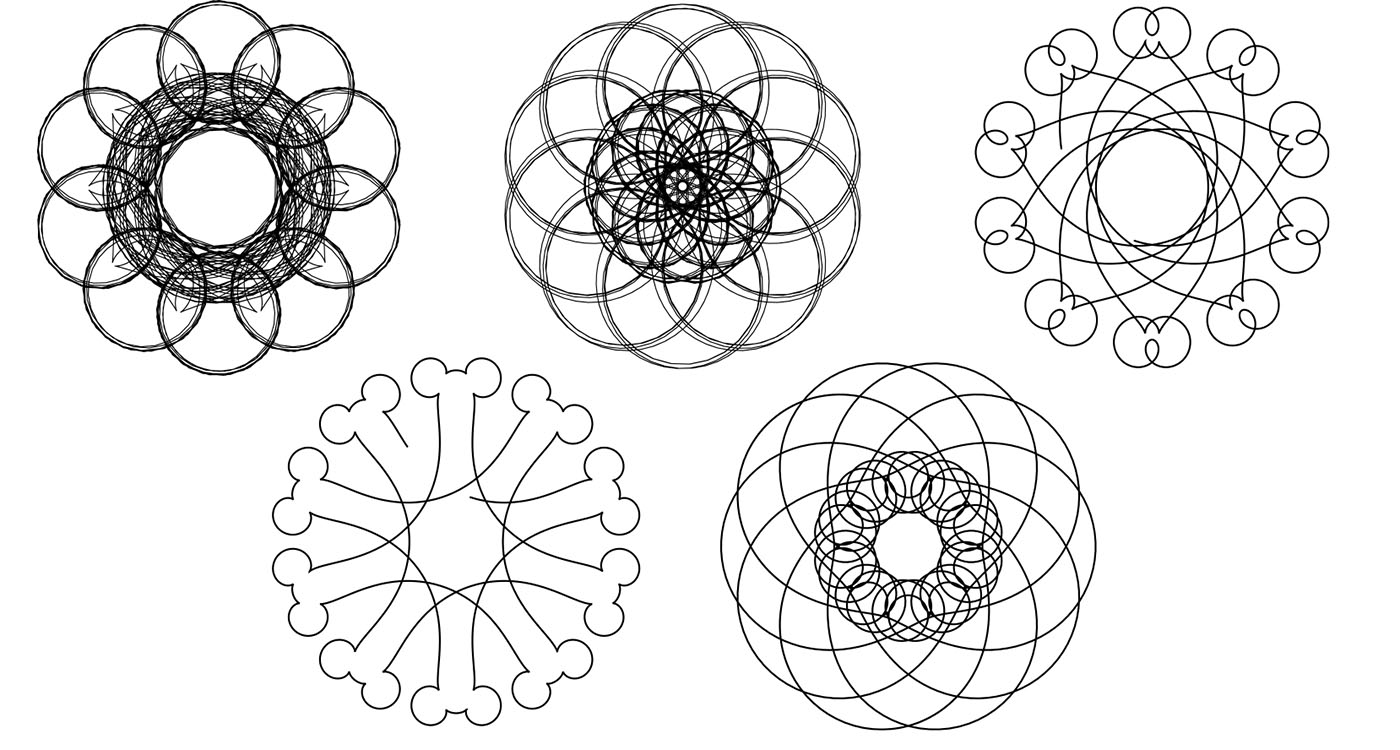
Figure 5. Schrödinger potentials \(p = a + b~cos~t + c~cos~2t\) represented as equivalent bike paths for different choices of \(a\), \(b\), \(c\).

References

[1] V.I. Arnold, Remarks on the perturbation theory for problems of Mathieu type, Russ. Math. Surveys, 38 (1983).
[2] H.W. Broer and C. Simo, Resonance tongues in Hill’s equations: A geometric approach, J. Differential Equations, 166:2 (2000), 290–327.
[3] R.L. Foote, Geometry of the Prytz planimeter, Rep. Math. Phys., 42:1–2 (1998), 249–271.
[4] R.L. Foote, M. Levi, and S. Tabachnikov, Tractrices, bicycle tire tracks, hatchet planimeters, and a 100-year-old conjecture, Amer. Math. Monthly, 120:3 (2013), 199–216.
[5] M. Levi, Geometry and physics of averaging with applications, Phys. D, 132 (1999), 150–164.
[6] M. Levi, Stability of the inverted pendulum—A topological explanation, SIAM Rev., 30 (1988), 639–644.
[7] M. Levi, Schrödinger’s equation and bike tracks—A connection, 2014; http://arxiv.org/pdf/1405.1741.pdf.
[8] M. Levi and S. Tabachnikov, On bicycle tire tracks geometry, Menzin’s conjecture, and oscillation of unicycle tracks, Exp. Math., 18:2 (2009),173–186.
[9] D.M. Levy and J.B. Keller, Instability intervals of Hill’s equation, Comm. Pure Appl. Math., 16 (1963), 469–476.
[10] W. Paul, Electromagnetic traps for charged and neutral particles, Rev. Modern Phys., 62 (1990), 531–540.
[11] M.I. Weinstein and J.B. Keller, Asymptotic behavior of stability regions for Hill’s equation, SIAM J. Appl. Math., 47 (1987), 941–958.
Mark Levi ([email protected]) is a professor of mathematics at Pennsylvania State University.