By Alexandre Em and Martin Vohralik
Systems of nonlinear algebraic equations arise in numerous applications of scientific computing. Iterative linearizations, with the Newton method as a prominent example (see, for example, [5]), are extensively used for the approximate solution of such systems. At each step of an exact Newton method, a system of linear algebraic equations needs to be solved. To alleviate the computational burden, the solution of this linear system can be approximated, typically by employing some early stopping criterion within an iterative linear algebraic solver. This is the essence of the so-called inexact Newton method. A crucial question is when the linear algebraic solver should be stopped. Is it possible to speed up the calculation with a suitably chosen algebraic stopping criterion? Answers via a priori limit theory have been suggested (see [1] and the references therein).
The situation becomes more intricate when the system of nonlinear algebraic equations results from the discretization of some nonlinear partial differential equation. In this context, three sources of error are inevitable: algebraic error, linked to the linear algebraic solver, linearization error, linked to the linearization iteration, and discretization error. It is then natural to envisage an early stopping criterion for the Newton iteration itself. Intuitively, converging the iterative linear and nonlinear solvers to machine precision does not seem to be necessary. Devising stopping criteria for both solvers so as to balance the three error components is not straightforward and, to our knowledge, such criteria have relied to date essentially on heuristics.
In [3], following [2, 4], we identified and estimated separately the three error components via the theory of a posteriori error estimates for nonlinear diffusion PDEs. Within this theory, we have used equilibrated flux reconstructions, originating in the pioneering work of Prager and Synge [6]. The twofold advantage of this approach is to deliver guaranteed, fully computable error estimates, a key issue for the conception of practical stopping criteria, and to allow for a unified theory encompassing most discretization schemes. We then devised and analyzed stopping criteria stipulating that there is no need to continue with the algebraic solver iterations once the linearization or discretization error components start to dominate, and no need to continue with the linearization iterations once the discretization error component starts to dominate. We call the resulting algorithm an adaptive inexact Newton method.
To illustrate the idea, we consider the following nonlinear diffusion PDE: Find \(u : \Omega \rightarrow \mathbb{R}\) such that
\[\begin{equation}
\nabla \cdot \boldsymbol{\sigma}(u,\nabla u) = f \qquad \mathrm{in}~ \Omega, \qquad \qquad \mathrm{(1a)} \\
u = 0 \qquad \qquad \qquad \mathrm{on}~ \partial \Omega, \qquad \qquad \mathrm{(1b)}
\end{equation}\]
where \(\Omega \subset \mathbb{R}^d, d \geq 2\), is a polygonal (polyhedral) domain (an open, bounded, and connected set), \(f : \Omega \rightarrow \mathbb{R}\) a given source term, and \(\boldsymbol{\sigma} : \mathbb{R} \times \mathbb{R}^d \rightarrow \mathbb{R}^d\) the nonlinear flux function. We let \(u^{k,i}_{h}\) be a numerical approximation of \(u\) obtained on a computational mesh of \(\Omega\), at the linearization step \(k\) and algebraic solver step \(i\). Up to higher-order terms on the right-hand side, our a posteriori error estimate takes on the general form
\[\begin{equation}\tag{2}
J_u(u^{k,i}_{h}) \leq \eta^{k,i} \leq \eta^{k,i}_{\mathrm{disc}} + \eta^{k,i}_{\mathrm{lin}} + \eta^{k,i}_{\mathrm{alg}}
\end{equation} \]
for a suitable error measure \(J_{u}(u^{k,i}_{h})\). Here, the overall estimator \(\eta^{k,i}\) as well as the estimators of the three error components \(\eta^{k,i}_{\mathrm{disc}}\), \(\eta^{k,i}_{\mathrm{lin}}\), and \(\eta^{k,i}_{\mathrm{alg}}\) are fully computable. Our stopping criteria can be formulated for the linear and nonlinear solvers, respectively, as
\[\begin{equation}\tag{3}
\eta^{k,i}_{\mathrm{alg}} \leq \gamma_{\mathrm{alg}}\mathrm{max}\{\eta^{k,i}_{\mathrm{disc}}, \eta^{k,i}_{\mathrm{lin}}\}, \\
\eta^{k,i}_{\mathrm{lin}} \leq \gamma_{\mathrm{lin}}\eta^{k,i}_{\mathrm{disc}},
\end{equation}\]
where the values of the parameters \(\gamma_{\mathrm{alg}}\) and \(\gamma_{\mathrm{lin}}\) are set by the user, typically to a small percentage. From a mathematical viewpoint, an important result is that, under our stopping criteria, there exists a generic constant \(C\) such that, up to higher-order terms on the right-hand side,
\[\begin{equation}\tag{4} \eta^{k,i}_{\mathrm{disc}} + \eta^{k,i}_{\mathrm{lin}} + \eta^{k,i}_{\mathrm{alg}} \leq CJ_u(u^{k,i}_{h}), \end{equation}\]
which is called efficiency and, together with (2), proves the equivalence of the error measure \(J_{u}(u^{k,i}_{h})\) with our estimates. Moreover, as \(C\) is independent of the mesh size \(h\), the domain \(\Omega\), and the nonlinear function \(\boldsymbol{\sigma}\), the a posteriori error estimate is robust. The bounds (2) and (4) are established for an error measure \(J_{u}(u^{k,i}_{h})\) based on a dual norm of the difference between the exact flux \(\boldsymbol{\sigma}(u,\nabla u)\) and the approximate flux \(\boldsymbol{\sigma}(u^{k,i}_{h}, \nabla u^{k,i}_{h})\). In numerical results for the nonlinear \(p\)-Laplace equation, that is, \(\boldsymbol{\sigma}(u, \nabla u) = -|\nabla u|^{p-2}\nabla u\) for a real number \(p > 1\) in (1), \(J_{u}(u^{k,i}_{h})\) is very close to the Lebesgue norm of the flux difference \(||\boldsymbol{\sigma}(u,\nabla u) − \boldsymbol{\sigma}(u^{k,i}_h, \nabla u^{k,i}_h)||_{q,\Omega}\), with \(q = p/(p − 1)\). This error measure is important from a physical viewpoint, as the underlying PDE expresses a conservation principle by means of a balance law for the fluxes. The derivation of a posteriori error estimates for alternative error measures, e.g., in a goal-oriented setting, is an active area of research.
Figure 1 shows a comparison of results for the exact, inexact, and adaptive inexact Newton methods in the example of a nonlinear \(p\)-Laplace equation, with discretization by the Crouzeix–Raviart nonconforming finite element method, Newton linearization, and a conjugate gradient linear solver with diagonal preconditioning. The behavior of the overall error measure \(||\boldsymbol{\sigma}(u,\nabla u) − \boldsymbol{\sigma}(u^{k,i}_h, \nabla u^{k,i}_h)||_{q,\Omega}\) as a function of the number of degrees of freedom is quite similar for the three methods. This means that our early stopping criteria do not influence the overall error. What differs is the level below which the “side” (algebraic and linearization) errors are forced to decrease; in our approach, the user specifies this by means of (3). We used \(\gamma_{\mathrm{alg}} = \gamma_{\mathrm{lin}} = 0.3\).
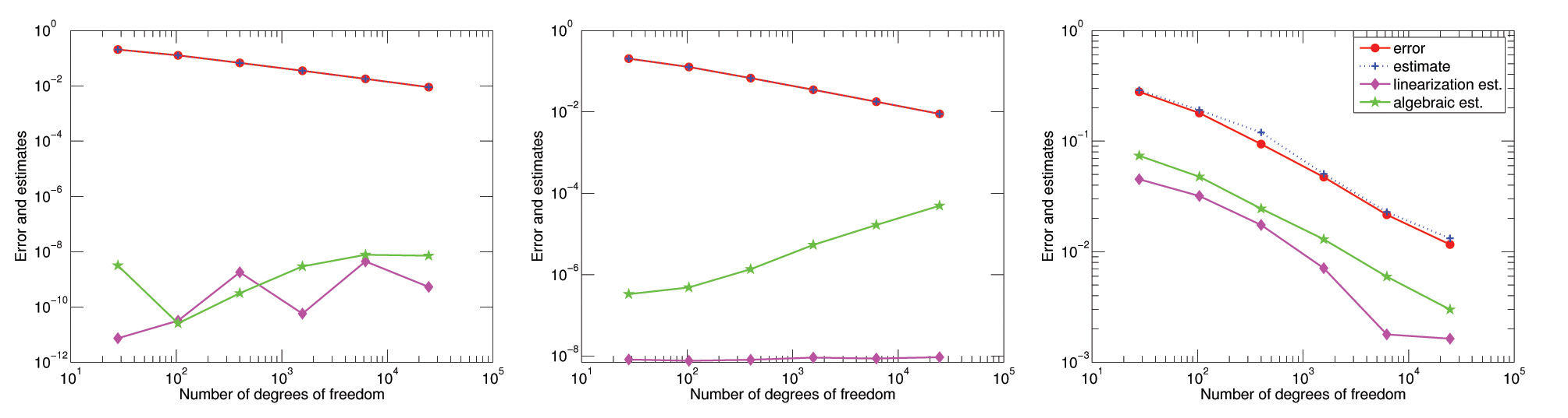
Figure 1. Error and estimates on a series of uniformly refined meshes with the exact Newton (left), inexact Newton (middle), and adaptive inexact Newton (right) methods.
|
The left panel of Figure 2 provides further insight into the dependence of the error and of our estimates on the Newton iterations. The error and all but the linearization estimates start to stagnate after the linearization error ceases to dominate. Whereas the exact Newton method (with a convergence criterion of 10−8) needs 20 iterations, we can safely stop after 11 iterations in our approach. The middle panel of Figure 2 presents similar plots for the CG iterations. Our adaptive algorithm stops after 32 iterations, whereas the exact method (with a convergence criterion of 10−8) needs about 650 iterations. The total number of algebraic solver iterations required per refinement level is displayed in the right panel of Figure 2. On the last mesh, the inexact Newton method achieves a sixfold speedup compared with the exact Newton method (8690 vs. 1470 iterations). Our adaptive inexact Newton method achieves a further fivefold speedup (306 vs. 1470 iterations).
|
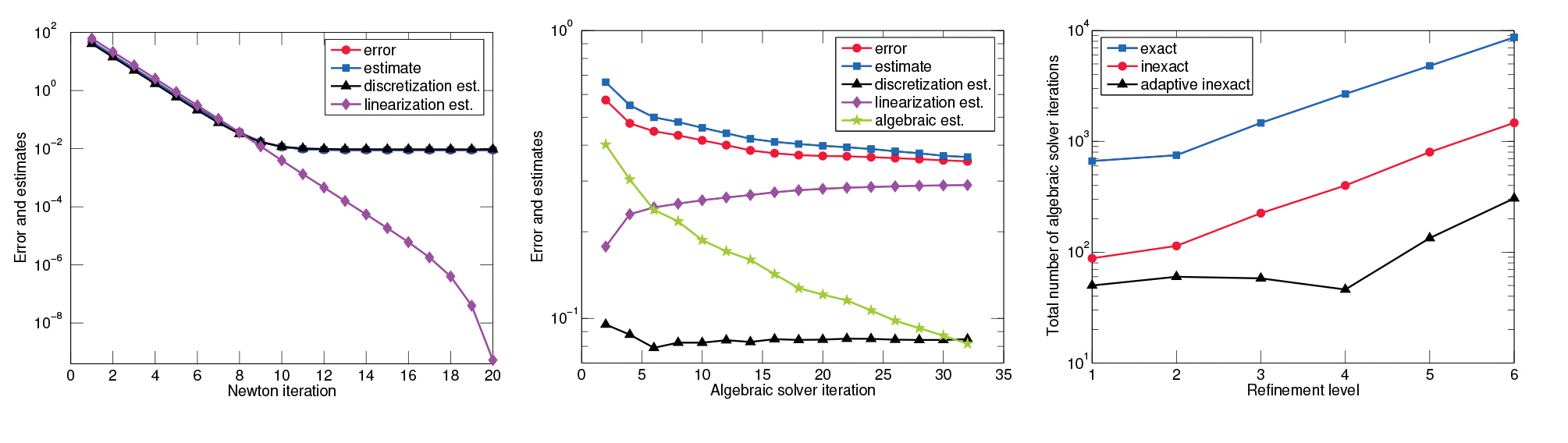
Figure 2. Error and estimates as a function of: Newton iterations, 6th-level uniformly refined mesh (left); preconditioned conjugate gradient iterations in the 8th Newton step on the 6th-level uniformly refined mesh (middle); and total number of linear solver iterations per uniform mesh refinement level (right).
|
In Figure 3, we illustrate our adaptive inexact Newton method in conjunction with adaptive mesh refinement, still for the nonlinear \(p\)-Laplace equation. With local, elementwise stopping criteria, the predicted error distribution typically matches the actual one quite nicely, as illustrated in Figure 3. The figure also shows the adaptive mesh refinement triggered by a corner singularity. This stems from a theoretical result asserting the local efficiency of our estimates that is formulated by means of a mesh-localized version of (4).
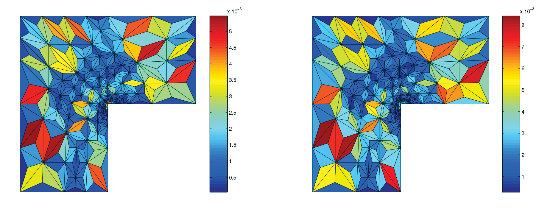
Figure 3. Estimated (left) and actual (right) error distribution, 5th-level adaptively refined mesh.
|
In conclusion, we advocate that only the necessary number of algebraic solver iterations at each linearization step, and only the necessary number of linearization iterations should be carried out within an adaptive inexact Newton method. This typically leads to important computational savings, further increased with the addition of mesh adaptivity, thereby paving the way to a complete adaptive strategy. The driving force is a posteriori estimates that ensure a guaranteed and robust error upper bound. More details on our approach can be found in [3].
References
[1] S.C. Eisenstat and H.F. Walker, Globally convergent inexact Newton methods, SIAM J. Optim., 4 (1994), 393–422.
[2] L. El Alaoui, A. Ern, and M. Vohralík, Guaranteed and robust a posteriori error estimates and balancing discretization and linearization errors for monotone nonlinear problems, Comput. Methods Appl. Mech. Engrg., 200 (2011), 2782–2795.
[3] A. Ern and M. Vohralík, Adaptive inexact Newton methods with a posteriori stopping criteria for nonlinear diffusion PDEs, HAL Preprint 00681422 v2, submitted for publication, 2012.
[4] P. Jiránek, Z. Strakoš, and M. Vohralík, A posteriori error estimates including algebraic error and stopping criteria for iterative solvers, SIAM J. Sci. Comput., 32 (2010), 1567–1590.
[5] L.V. Kantorovich, Functional analysis and applied mathematics, Uspekhi Mat. Nauk, 3 (1948), 89–185.
[6] W. Prager and J.L. Synge, Approximations in elasticity based on the concept of function space, Quart. Appl. Math., 5 (1947), 241–269.
Alexandre Ern is a professor of scientific computing at Ecole des Ponts ParisTech, Université Paris-Est, and an associate professor of numerical analysis and optimization at Ecole Polytechnique. Martin Vohralík is a senior researcher at INRIA Paris-Rocquencourt.