A Measure of Morphodynamics

By Mattia Serra and L. Mahadevan

One of the grand challenges of modern biology is understanding the way in which a complex, multicellular organism arises from a single cell via spatiotemporal patterns that are repeatable and reproducible across the tree of life. As the organism grows, its cells change their number, size, shape, and position in response to genetic, chemical, and mechanical cues (see Figure 1a). Four-dimensional microscopy (three spatial dimensions and time) is beginning to illuminate how these cues impact the fate of cells and the geometric form of tissues and organs that constrain and enable function at multiple scales [3]. Even though individual cells might seem to move chaotically, the large-scale, collective cell movements within tissues resemble a choreographed ballet and raise a few natural questions:

1. How can we quantify the patterns and predict the formation of different organ systems?
2. How can we understand these patterns from a biophysical and biochemical perspective as a function of the way in which cells divide, grow, and move in response to environmental cues? 
3. How can we control these movements to intervene and correct pathological development or guide tissue development in situations like organoid formation?

Figure 1. Frame-invariant description of cellular flows. 1a. Sketch of bottom-up and top-down approaches to cell motion. Bottom-up approaches study local mechanisms that drive cells, while top-down approaches study patterns of cell motion that are caused by local and global driving mechanisms. The dynamic morphoskeleton uncovers the centerpieces of cell trajectory patterns in space and time. 1b. Snapshots of a simple analytic velocity field (blue) and its Lagrangian particle positions (green). The black dot marks the position of a particle that began at the black \(x\) marker at time 0. The frame-dependent velocity field suggests the presence of a vortical structure while the tissue undergoes exponential stretching. Figure courtesy of [6].

Here we focus on the properly invariant quantification of large-scale cellular movements and draw inspiration from the study of objective transport barriers in hydrodynamics [2, 5]. Just as it is more meaningful to focus on the large-scale coherent structures in a complex flow rather than track individual particles, we believe that it is useful to quantify the large-scale motions that characterize tissue morphogenesis. Any framework that aims to analyze spatiotemporal trajectories in morphogenesis requires a self-consistent description of cell motion that is independent of the choice of reference frame or parametrization. This objective (frame-invariant) description of cell patterns ensures that the material response of a deforming continuum—e.g., a biological tissue—is independent of the observer [7].

One can quantify this idea mathematically by considering two reference frames that describe cellular flows and are related to each other via the transformation \(\boldsymbol{\bar{x}}(t)=\boldsymbol{Q}(t)\boldsymbol{x}(t) + \boldsymbol{b}(t)\), where \(\boldsymbol{Q}(t),\boldsymbol{b}(t)\) are a time-dependent rotation matrix and translation vector respectively. A quantity is objective (frame invariant) if the corresponding descriptions in both frames transform appropriately: scalars \(c(t)\) (e.g., concentration) must remain the same with \(\bar{c}(t)=c(t)\); vectors \(\boldsymbol{v}(t)\) (e.g., velocity field) must transform via the rule \(\boldsymbol{\bar{v}}(t)=\boldsymbol{Q}(t)\boldsymbol{v}(t)\); second-order tensors \(\boldsymbol{A}(t)\) (e.g., strain rate) must transform via the rule \(\boldsymbol{\bar{A}}(t)=\boldsymbol{Q}(t)\boldsymbol{A}(t)\boldsymbol{Q}^T(t)\); and so forth [7]. It is thus immediately apparent that objects like velocity fields, streamlines, and vorticity—which are typical outputs from microscopy following some elementary image analyses—are frame dependent. Therefore, any metrics that are based on these objects for comparative purposes are likely erroneous, owing to their inability to remove dependence on artifacts that are associated with variations in the choice of reference frames (see Figure 1b). Indeed, most Eulerian approaches that characterize fluid or cellular flows suffer from this flaw, despite having served as workhorses for a long time [1, 5]. So, how can we do better?

Figure 2. Attractors and repellers organize cell motion. 2a. Illustration of the attracting and repelling Lagrangian coherent structures (LCSs) over the time interval \([t_0,t]\). 2b. The forward finite-time Lyapunov exponent (FTLE) measures the maximum separation \(\delta\boldsymbol{x}_t\) over the time interval \([t_0,t]\) between two initially close points in the neighborhood \(\boldsymbol{x}_0\). A forward-time FTLE ridge—a set of points with high FTLE values—marks a repelling LCS; nearby points from opposite sides of the ridge experience the maximum separation over \([t_0,t]\), \(t>t_0\). 2c. A backward-time FTLE ridge demarcates an attracting LCS — i.e., a distinguished curve at the final time that has attracted initially distant particles. Figure adapted from [6].

A Lagrangian view that integrates over the history of cellular movements in time can clearly distinguish the way in which cells move apart or together, and ultimately provides a better perspective on cellular and tissue fate. This approach has successfully unraveled the complexity of passive fluid flows in problems that range from microfluidic mixing to atmospheric polar vortices using the notion of Lagrangian coherent structures (LCSs) [2]. Hyperbolic LCSs are time-evolving attracting and repelling manifolds that shape the overall spatiotemporal patterns in complex dynamical systems. In the context of morphogenesis, the dynamic morphoskeleton is the collection of attracting and repelling LCSs. From a practical perspective, we can compute these structures in terms of the largest finite-time Lyapunov exponent (FTLE), which is defined as

\[\Lambda^t_{t_0}(\boldsymbol{x}_0)=\frac{1}{|T|}\ln\left(\underset{\delta\boldsymbol{x}_0}{\max} \frac{\left|\overbrace{\triangledown\boldsymbol{F}^t_{t_0}(\boldsymbol{x}_0)\delta\boldsymbol{x}_0}^{\delta\boldsymbol{x}_t}\right|}{|\delta\boldsymbol{x}_0|}\right).\]

Here, \(\boldsymbol{F}^t_{t_0}(\boldsymbol{x}_0)=\boldsymbol{x}_0+\int^t_{t_0}\boldsymbol{v}(\boldsymbol{F}^\tau_{t_0}(\boldsymbol{x}_0), \tau)d\tau\) is the Lagrangian flow map that is induced by cell velocities. \(\Lambda^t_{t_0}(\boldsymbol{x}_0)\) characterizes the maximum rate of separation of points in a neighborhood of \(\boldsymbol{x}_0\)—denoted by the infinitesimal vector \(\delta\boldsymbol{x}_0\)—during the time window \([t_0,t]\) (see Figure 2). The FTLE has a natural interpretation in continuum mechanics and is related to the largest eigenvalue of the Cauchy-Green strain tensor [7], therefore serving as a natural invariant measure of deformation in a continuous medium.

By choosing to integrate either forwards or backwards in time, one can delineate manifolds that are zones of attraction or repulsion over a given time interval; doing so establishes an organizing skeleton for the flow pattern (see Figure 2). The resulting dynamic morphoskeleton is frame invariant, easy to compute, and robust to noise and loss of local data because of its (integrated) averaging property [6].

When deploying this approach on light-sheet microscopy data from the embryo of a normally-developing chick that involves \(\sim 10^5\) cells (see Figure 3a) [4], we see that the dynamic morphoskeleton consists of two repellers—critical boundary regions across which cells will likely assume different fates—and one attractor (see Figure 3b). Repeller 1 marks a dynamic boundary between the embryonic and extra-embryonic regions. By contrast, repeller 2 marks the anterior-posterior boundary of a characteristic feature that is known as the primitive streak (PS): a zone of strong cellular convergence (an attractor) during early embryogenesis. First, we note that repellers remain invisible to Eulerian and Lagrangian tools that researchers use in multicellular flows (see Animation 1). This fact may explain why repellers appear to be undocumented in the literature, despite their relevance for cell fate acquisition.

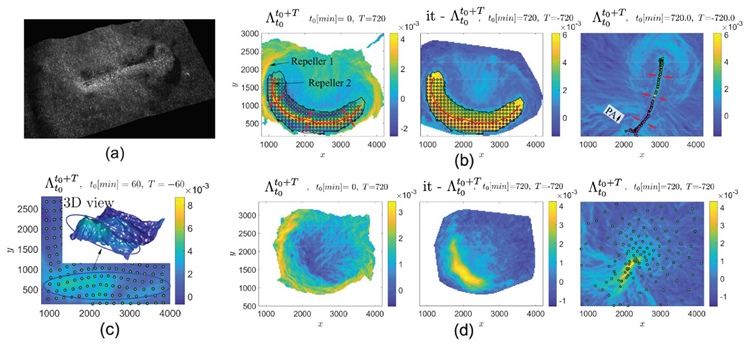
Figure 3. Dynamic morphoskeletons in chicken gastrulation. 3a. Light-sheet microscopy image of a chick epiblast during the primitive streak (PS) formation. 3b. Left: \(FW \, FTLE^{12h}_0\) highlights two repelling Lagrangian coherent structures (LCSs). Right: \(BW \, FTLE^0_{12h}\) highlights the attracting LCS that corresponds to the formed PS. Center: \(BW \, FTLE^0_{12h}\) field in the right panel is passively transported to the initial time; this marks the initial position of the mesendoderm precursor cells—bounded by the solid black line—that eventually form the PS. Cells that begin on different sides of repeller 2 form the anterior and posterior part of the PS. The finite-time Lyapunov exponent (FTLE) has units 1/min, and the axis units are in µm. The time evolution of the FTLE fields and cell positions for different \(T\) are available in Animation 1. 3c. \(BW \, FTLE^0_{1h}\) ridge highlights the PS’s early footprint (blue ellipse) using only the first hour of data when the cells (green dots)—initially released on a uniform rectangular grid—have barely moved. 3d. The same situation as 3b for a chick embryo that is treated with a critical diffusible morphogen (FGF) receptor inhibitor. See Animation 2 for the time evolution of the FTLE fields and cell positions for different \(T\). Figure 3a courtesy of Cornelius Weijer, 3b-3d adapted from [6].

Second, we notice that just an hour after cells have barely started to move, the dynamic morphoskeleton captures the PS’s early footprint — well before it is actually visible to conventional tools (see Figure 3c). This approach can also detect preliminary signatures of abnormal development. Use of a drug to inhibit the presence of a critical diffusible morphogen (FGF) that is required for early gastrulation causes the PS formation to fail (see Figure 3d) and results in a lack of anterior-posterior cell differentiation, which is quantified by the loss of repeller 2 (evident in the left panels of Figure 3b and 3d, and in Animation 2). Similar analysis of a whole curved embryo of a developing fruit fly with roughly 6,000 cells allows us to visualize how the attractors and repellers characterize the motions that lead to gastrulation in both normal and pathological development [6].

The enormous amounts of data that are rapidly becoming available from large-scale imaging of biological development require properly invariant methods of analysis. The aforementioned approach—which integrates local (cell-based) and nonlocal (neighborhood/tissue-based) cues—provides a step in the right direction. The dynamic morphoskeleton sets the geometric stage for uncovering the dynamic organizers of cellular movements and tissue form; it also provides a lens for uncovering the underlying relevant mechanisms at play. When we combine the morphoskeleton with the ability to track and manipulate gene expression levels, mechanical forces, etc., perhaps we will be able to determine the biophysical mechanisms that underlie normal and pathological morphogenesis and move a little closer to answering one of the grand questions of modern biology.

This article is based on Mattia Serra's minisymposium presentation at the 2019 SIAM Conference on Applications of Dynamical Systems, which took place in Snowbird, Utah.

Mattia Serra is an assistant professor of physics at the University of California, San Diego. He was previously a Schmidt Science Fellow at Harvard University. L. Mahadevan is a professor of applied mathematics, physics, and organismic and evolutionary biology at Harvard University.

References

[1] Blanchard, G.B., Kabla, A.J., Schultz, N.L., Butler, L.C., Sanson, B., Gorfinkiel, N., …, Adams, R.J. (2009). Tissue tectonics: Morphogenetic strain rates, cell shape change and intercalation. Nat. Methods, 6(6), 458-464.
[2] Haller, G. (2015). Lagrangian coherent structures. Ann. Rev. Fluid Mech., 47, 137-162.
[3] McDole, K., Guignard, L., Amat, F., Berger, A., Malandain, G., Royer, L., …, Keller, P.J. (2018). In toto imaging and reconstruction of post-implantation mouse development at the single-cell level. Cell, 175(3), 859-876.
[4] Rozbicki, E., Chuai, M., Karjalainen, A.I., Song, F., Sang, H.M., Martin, R., …, Weijer, C.J. (2015). Myosin-II-mediated cell shape changes and cell intercalation contribute to primitive streak formation. Nat. Cell Biol., 17(4), 397-408.
[5] Serra, M., & Haller, G. (2016). Objective Eulerian coherent structures. Chaos, 26(5), 053110.
[6] Serra, M., Streichan, S., Chuai, M., Weijer, C., & Mahadevan, L. (2020). Dynamic morphoskeletons in development. Proc. Natl. Acad. Sci., 117, 11444-49.
[7] Truesdell, C., & Noll, W. (2004). The non-linear field theories of mechanics. New York, NY: Springer.