Typical dynamical systems can either have simple trajectories, such as steady states or periodic or quasiperiodic orbits, or they can be chaotic. While simple behavior is well understood, chaos is defined in so many different ways that is it confusing and difficult to get a reasonable answer to the simple question: What is the definition of chaos? We assert that this is the wrong question to ask.
Chaos does not have a satisfactory single mathematical definition, not because it is not a single mathematical concept, but rather because it has many mathematical manifestations in many different situations. In this regard, we are reminded of the 2500-year-old parable of the blind monks and the elephant. Each monk touches a different part of the elephant; a monk feeling a tusk thinks the elephant is a spear, while others encounter different manifestations of the elephant—a rope-like tail, perhaps, or column-like legs. When we observe a chaotic system, we are blind to the enormity of the concept and observe only a limited number of aspects of the system’s chaotic nature.
In this article we discuss a variety of the manifestations and mathematical definitions of chaos. Our underlying message is that although it is possible to find pairs of definitions, one of which indicates that a system is chaotic and the other that it is not, this phenomenon is the exception, rather than the rule. We conjecture that, typically, the different forms of chaos are equivalent.
Arguably, the earliest observation of mathematical chaos occurred in the context of Newtonian mechanics. Henri Poincaré wrote a proof of the stability of the solar system, a result for which he won a substantial prize from King Oscar II of Sweden in 1890. After the prize was awarded, Lars Edvard Phragmén pointed out a substantial omission: Poincaré had assumed that only simple behavior could occur in a situation in which, in fact, it is possible to have chaotic behavior and what is now known as a transverse homoclinic orbit. In particular, there is a Cantor set of points with the property that the trajectory through almost any one of them occasionally comes arbitrarily close to that steady state both forward and backward in time, but with large excursions along the way.
Poincaré’s proof of the stability of the solar system completely collapsed, and the question remains open today (although the high likelihood of the survival of the planets in their orbits has been verified numerically to the expected time of the sun’s demise). Poincaré then undertook a major rewrite of the paper, in the course of which he discovered the underlying complexity of dynamical systems. In his words, “If one seeks to visualize the pattern formed . . . a chain-link network of infinitely fine mesh . . . one will be struck by the complexity. . ., which I am not even attempting to draw” [3]. Thankfully, the existence of computers makes it possible to depict this situation (which is shown in Figure 1).
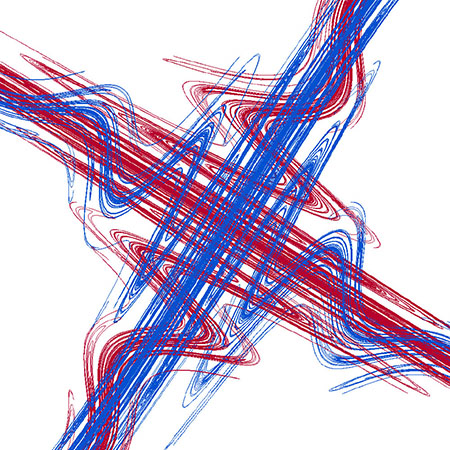
Figure 1. A homoclinic tangle with the chaotic complexity described by Poincaré.
|
Following this path of ideas, Stephen Smale showed in 1967 that even in a simple two-dimensional map known as a horseshoe map, one sees the same complexity as in transverse homoclinic orbits; in fact, horseshoe maps are embedded in any system containing a transverse homoclinic orbit. This aspect of chaos is useful when visualization is difficult but analysis is tractable, as for delay differential equations and partial differential equations. Chaos of this type can often be transient—that is, it cannot be observed through direct simulations of a trajectory or in physical experiments. Furthermore, the characterization is not quantitative.
In the course of numerical experiments for models of two very different natural systems, Yoshisuke Ueda (in 1961) and Edward Lorenz (in 1963) observed a robust but highly irregular topology in the trajectories of the systems. This “fractal topology” is a hallmark of attracting chaotic systems known as strange attractors; their measurement has since been made more precise in the form of attractor-dimension calculations. A general definition of strange attractors is still lacking, however, except for the subtype of rank-one attractors. Transverse homoclinic orbits often play a key role in shaping the geometry of strange attractors, and these concepts have been rigorously shown to be tightly related in many subclasses of systems.
Rather than providing full knowledge of a system, experiments often give rise to time-series data. In 1975, Jerry Gollub and Harry Swinney demonstrated that the time-series data from Taylor–Couette fluid flow experiments had the chaotic hallmark of a broad power spectrum. In fact, the closely related Lyapunov exponent is the current most commonly used metric for characterizing chaos; using added information about the behavior of nearby orbits, the Lyapunov exponent indicates the degree of stretching along solutions. For experimental high-dimensional chaos, it is not possible in general to observe this stretching. The concept of stretching also appears in the definition of scrambled sets of Li and Yorke. Aside from stretching, another way to measure chaos is the possession of positive entropy. If the number of “distinct” orbits of period \(n\) is proportional to \(a^n\), then the entropy is proportional to \(\log(a)\). As with chaos, there are a variety of types of entropy. Each of the above-mentioned concepts can be shown to be distinct, although they appear to overlap in all but rather extreme cases, as discussed in [2].
The importance of non-attracting chaos is often overlooked, as it cannot be seen either by direct simulation or experimental observation. This behavior, though not stable, can organize the underlying behavior of the system and can be robust under changes to the system parameters. Such is the case for chaotic saddles. Figure 2 (see page 1), for example, shows the basins of eight attractors for the forced–damped pendulum. The eight attractors are simply periodic and fixed points. The chaotic saddle on the boundary of the basins causes the geometric complexity. The progression of the basins as the forcing changes can be seen in our YouTube video [4].
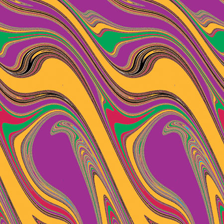
Figure 2. Eight basins of attraction for the forced–damped pendulum. The geometic complexity of the basins results from the chaos on their boundaries.
|
Each manifestation or definition of chaos mentioned here comes with its own settings in which it can be verified, and with its own strengths and shortcomings, in terms of both numerical and theoretical uses. It is true that the non-equivalence of these mathematically precise formulations can be shown, but we choose to focus on the similarities, reiterating that the concept of chaos is too big for one single mathematical definition to suffice. We end by quoting a statement made during the controversy about Pluto as it was stripped of planethood, but which applies just as well to the chaos definition controversy: “Nature abhors a definition. Try to lock something into too small a box, and I guarantee nature will find an exception” [1].
References
[1] M. Brown,
How I Killed Pluto and Why It Had It Coming, Random House, New York, 2010.
[2] B. Hunt and E. Ott,
Defining chaos, Chaos, to appear;
http://arxiv.org/abs/1501.07896.
[3] H. Poincaré,
New Methods of Celestial Mechanics, Vol. 13, American Institute of Physics, College Park, Maryland, 1993.
[4] E. Sander and J. Yorke,
Pendulum gyrations, 2014;
http://youtu.be/JyhaHyCvgw4 and
http://math.gmu.edu/˜sander/EvelynSite/pendulum-gyrations.html.
[5] E. Sander and J. Yorke,
The many facets of chaos, Internat. J. Bifur. Chaos Appl. Sci. Engrg., 25 (2015), 1530011-1-15.
This article is a summary of our recent paper [5] and is based on the talk Evelyn Sander gave at the 2015 SIAM Conference on Applications of Dynamical Systems. Readers can find a more substantial reference list in the paper.
Evelyn Sander is a professor of mathematics at George Mason University. Jim Yorke is a Distinguished University Research Professor of Mathematics and Physics at the University of Maryland, College Park.