The Rational Krylov Toolbox

By Stefan Güttel

Rational Krylov methods have become an indispensable tool in the field of scientific computing. Originally invented for the solution of large, sparse eigenvalue problems, these methods have seen an increasing number of other uses over the last two decades. Example applications include model order reduction, matrix function approximation, matrix equations, nonlinear eigenvalue problems, and nonlinear rational least squares fitting.

Here I aim to provide a short introduction to rational Krylov methods, using the MATLAB Rational Krylov Toolbox (RKToolbox) for demonstration. The RKToolbox is freely available online and features an extensive collection of examples that users can explore and modify. The following text contains pointers to select RKToolbox examples, which are printed in typewriter font. Readers can also utilize these examples for teaching purposes, as they might serve as good starting points for computational coursework projects.

Rational Krylov: A Brief Introduction

A rational Krylov space is a natural generalization of the more widely known (standard) Krylov space. The latter is defined as

\[\mathcal{K}_m=\textrm{span}\{b,Ab,...,A^{m-1}b\},\]

where \(A\) is a square matrix and \(b\) is a nonzero vector of compatible size. We can represent every element in \(\mathcal{K}_m\) as a polynomial \(p(A)b\). On the other hand, a rational Krylov space is a linear space that is spanned by rational functions \(r(A)b\). For illustrative purposes, assume that we have three distinct complex numbers \(\xi_1\), \(\xi_2\), and \(\xi_3\) — all of which are different from \(A\)'s eigenvalues. We can then define the four-dimensional rational Krylov space as

\[\mathcal{Q}_4=\textrm{span}\{b,(A-\xi_1I)^{-1}b,(A-\xi_2I)^{-1}b,(A-\xi_3I)^{-1}b\}\tag1\]

(in artificial cases, \(\mathcal{Q}_4\) can have a dimension that is less than four, but we assume that this does not happen here). In order to work with \(\mathcal{Q}_4\) numerically, we compute an orthonormal basis with a method that is very similar to the standard Arnoldi algorithm. This method computes a matrix decomposition of the form

\[A\underbrace{[v_1,v_2,v_3,v_4]}_V \underbrace{\begin{bmatrix} \times & \times & \times \\ \times & \times & \times \\ & \times & \times \\ & & \times \end{bmatrix}}_K = \underbrace{[v_1,v_2,v_3,v_4]}_V \underbrace{\begin{bmatrix} \times & \times & \times \\ \times & \times & \times \\ & \times & \times \\ & & \times \end{bmatrix}}_H,\tag2\]

where the columns of \(V\) form an orthonormal basis of \(\mathcal{Q}_4\) and the rectangular four-by-three matrices \(H\) and \(K\)  are of upper Hessenberg form (i.e., all entries below the first subdiagonal are \(0\)).

The computation of \((2)\) requires the solution of three shifted linear systems with \(A\). This requirement is typically the computational bottleneck of rational Krylov methods, but there is potential for coarse-grain parallelism if we solve these systems simultaneously; more information is available in the RKToolbox example_parallel.html.

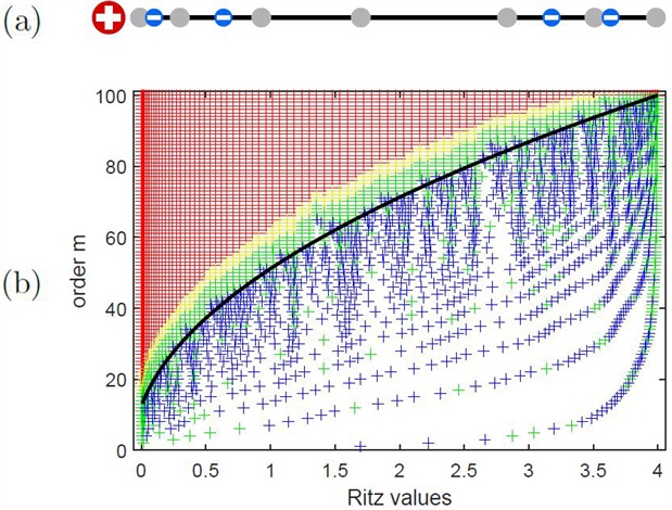
Figure 1. Electrostatic interpretation of rational Ritz values. 1a. Imagine that the eigenvalues of \(A\) (gray disks) are placed on a wire (black line). The \(m\)th-order Ritz values (blue disks) will then tend to distribute like electrons on the wire, satisfying the following properties: (i) Every two Ritz values are separated by at least one eigenvalue, (ii) the Ritz values repel each other, and (iii) they are attracted by an external field that is produced by the poles (red disk on the left); one can think of these poles as positive charges. Ritz values hence tend to find eigenvalues that are near the poles and in regions with few other eigenvalues. 1b. Ritz values (colored “plus” signs) of order \(m=1,2,...,100\) for the tridiagonal matrix A = gallery(‘tridiag’, 100) in MATLAB. All eigenvalues of \(A\) lie in the interval \([0,4]\) and all poles of the rational Krylov space are located at \(0\). The colors indicate a Ritz value’s distance to a closest eigenvalue of \(A\) and range from blue (not very close) to green and yellow and ultimately to red (extremely close). The region of converged Ritz values, which is depicted by the black curve, can be characterized analytically.

Eigenvalue Computations

Decompositions of the form \((2)\) play a central role in eigenvalue computations [4]. It turns out that eigenvalues of appropriate submatrices of \(H\) and \(K\)—so-called Ritz values—may actually approximate some of \(A\)'s eigenvalues quite well. This capability is completely analogous to the way in which we use the standard Arnoldi and Lanczos algorithms to approximate eigenvalues of large matrices. If \(A\) is a symmetric matrix, we even have a good theoretical understanding of which eigenvalues of \(A\) are well approximated by Ritz values [2]. Figure 1 illustrates a neat electrostatic interpretation of this concept. The RKToolbox provides examples for the numerical solution of linear and nonlinear eigenvalue problems at example_eigenproblems.html and example_nlep.html. 

Figure 2. Example of rational filter construction.

RKFUN Calculus

A useful feature of the decomposition in \((2)\) is that matrices \(H\) and \(K\) encode rational functions, or so-called RKFUNs. The RKToolbox uses this matrix representation to enable an array of numerical operations with rational functions. The object-oriented MATLAB implementation of RKFUNs was inspired by the Chebfun package [3]. In addition to root and pole finding, it is possible to add, multiply, and concatenate RKFUNs — as well as convert them into partial fraction, quotient, and continued fraction forms. We can implement all of these operations with established numerical linear algebra routines. For example, the conversion to continued fraction form utilizes the nonsymmetric Lanczos tridiagonalization process.

RKToolbox demonstrations of RKFUN calculus include example_rkfun.html, example_feast.html, and example_filter.html. Figure 2 is an example of rational filter construction.

 As Figure 3 illustrates, we can easily plot the filters with a command such as ezplot(butterworth, [0,2]). The elliptic filter—also known as the Cauer filter—is based on Zolotarev’s equioscillating rational functions, which are implemented in the RKToolbox’s gallery (a collection of special rational functions).

Figure 3. Rational filter functions that are constructed using RKFUN calculus.

Model Order Reduction

Model order reduction is one of the key drivers of research on rational Krylov methods. Interpolatory Methods for Model Reduction [1]—particularly chapters three and five therein—describes the way in which rational Krylov spaces serve as natural projection spaces for large-scale, linear time-invariant (LTI) dynamical systems. The iterated rational Krylov algorithm (IRKA) is of particular interest for the optimal interpolatory reduction of LTI systems in the \(\mathcal{H}_2\) norm. The RKToolbox contains several model order reduction problems, such as example_frequency.html, example_iss.html, and example_cdplayer.html.

Here I have provided a brief introduction to rational Krylov methods and referenced a number of applications, like eigenvalue problems and model order reduction. 

All figures are courtesy of the author.

References
[1] Antoulas, A.C., Beattie, C.A., & Güǧercin, S. (2020). Interpolatory methods for model reduction. In Computational science and engineering. Philadelphia, PA: Society for Industrial and Applied Mathematics.
[2] Beckermann, B., Güttel, S., & Vandebril, R. (2010). On the convergence of rational Ritz values. SIAM J. Matrix Analysis Appl., 31(4), 1740-1774.
[3] Driscoll, T.A., Hale, N., & Trefethen, L.N. (2014). Chebfun guide. Oxford, England: Pafnuty Publications.
[4] Ruhe, A. (1984). Rational Krylov sequence methods for eigenvalue computation. Linear Algebra Appl., 58, 391-405.

Stefan Güttel is a professor of applied mathematics at the University of Manchester and a Fellow of the Alan Turing Institute. He received SIAM’s 2021 James H. Wilkinson Prize in Numerical Analysis and Scientific Computing.