GRACE Satellite Data Delineates Changing Earth Surface
By James Case
This article is based on portions of a public lecture the author heard at the Aspen Center for Physics, Aspen, Colorado, in July 2012. The speaker, Ralph J. Cicerone, is an atmospheric scientist and current president of the U.S. National Academy of Sciences; the lecture was titled “Contemporary Climate Change as Seen Through Data.”
It has been known since the time of the French Revolution that the plumb lines observed at different points on the Earth’s surface are often “skew” to one another, meaning that they meet nowhere, much less at the planetary center of mass. Consequently, the Earth’s gravitational field differs in kind from those generated by simple point masses, spheres, or ellipsoids of uniform density. Until the advent of satellite technology, however, there was no practical way to determine the actual shape of the field. That’s why, in 1976, NASA launched the first LAGEOS satellite; it remains in orbit some 6000 kilometers above the Earth’s surface to this day, providing laser-assisted range measurements of remarkable accuracy to points of interest on the Earth’s surface. But because more accurate measurements can be made from satellites orbiting closer to ground level, NASA and the Deutsches Zentrum für Luft und Raumfahrt have joined forces in GRACE—the Gravity Recovery and Climate Experiment—which is designed to map the Earth’s gravitational field with previously unattained precision.
The knowledge to be gained from such an undertaking should prove extremely valuable. It will, among other things, help scientists to decide whether rising sea levels are due mainly to melting ice sheets, thermal expansion of the ocean water, or increasing salinity. It will also help them to separate the effects of gravity and ocean currents, and so to decide which shorelines should prepare for the most rapidly rising sea levels. Models have long predicted (and measurements begun to confirm) that sea levels will rise about twice as fast along shores like those of Virginia and southern California, where ocean currents are directed landward, as elsewhere along the east and west coasts of the U.S.
Already GRACE data has revealed the existence of the 300-mile-wide Wilkes Land crater in Antarctica, believed to have formed about 250 million years ago. It offers new ways of calculating ocean bottom pressures—as important to oceanography as atmospheric pressure is to meteorology. GRACE data has also been used to determine the water content of the soil in various agricultural regions, to analyze the movements of the Earth’s crust caused by the earthquake that created the 2004 tsunami in the Indian Ocean, and to measure “post-glacial rebound,” the ongoing process whereby the Earth’s crust is gradually returning to the shape it had before the last ice age, when “climate change” was responsible for coverage of much of the northern hemisphere with snow and ice to a depth of perhaps 200 miles.
The Earth’s gravitational field is the gradient field of a potential \(V(r,\theta,\lambda)\), where \(r, \theta, \lambda\) represent the radial distance, latitude, and longitude of a point on or above the surface. The function \(V\) can be expanded in spherical harmonics as follows:
\[\begin{equation}
V(r, \theta, \lambda) = \frac{GM}{R} \sum_{l=0}^{\infty} \sum_{m=0}^{l} (\frac{R}{r})^{l+1} \\
P_{lm} (\mathrm{sin}~ \theta)(C_{lm}~\mathrm{cos}(m\lambda)+S_{lm}~\mathrm{sin}(m\lambda)),
\end{equation}\]
where \(R\) is the Earth’s mean radius, \(M\) the mass of the Earth, \(G\) the universal gravitational constant, \(l\) and \(m\) are the spherical harmonic “degree” and “order,” \(P_lm\) is a “fully normalized” Legendre function, and \(S_lm\) and \(C_lm\) are the usual Stokes coefficients. The first few hundred of these can be obtained by numerical evaluation of standard integrals using GRACE data.
The equipotential surface that best approximates the mean ocean surface is known as the “geoid” of the Earth. Gauss introduced the term during the years he spent mapping the Duke of Brunswick’s ancestral lands, describing it as “the mathematical figure of the Earth.” Being an equipotential surface, it is everywhere perpendicular to the force of gravity, as determined by local plumb lines. Geoids are surprisingly irregular, though significantly less so than the Earth itself. Recent estimates deviate from the standard ellipsoidal approximation by little more than 100 meters (see Figure 1).
|
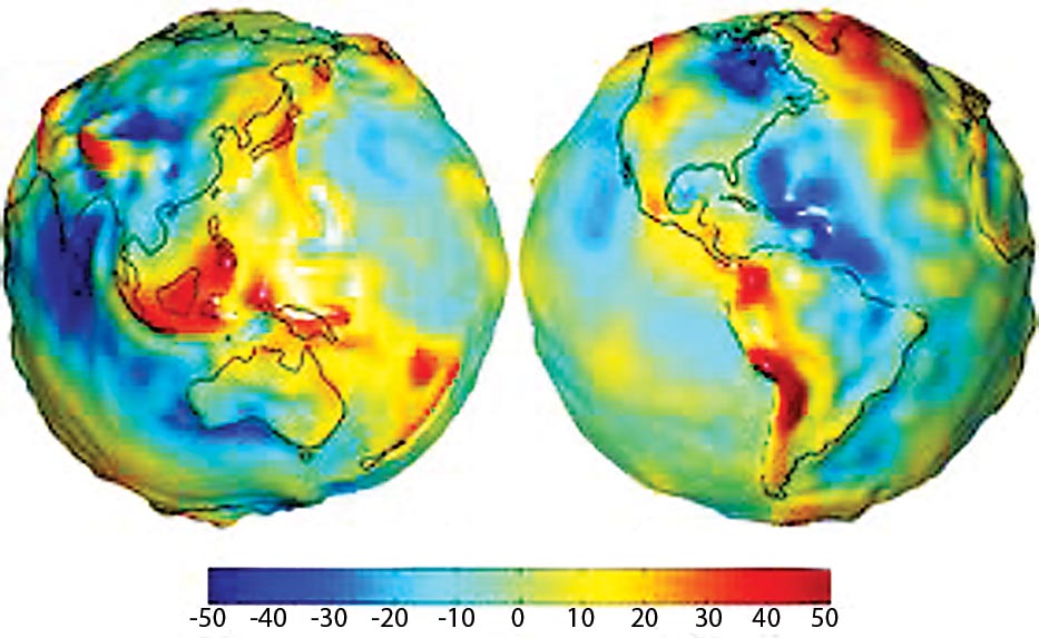
Figure 1. Three-dimensional visualization of geoid undulations, using units of gravity.
|
GRACE data is obtained from a pair of satellites—nicknamed Tom and Jerry—one trailing the other at a distance of about 220 kilometers in polar orbit some 500 kilometers above the Earth’s surface. Though that orbit has been deteriorating since March 2002, when the mission was launched, both are expected to remain in service at least until 2015. Circling the Earth 15 times a day, each overflies the equator once every 48 minutes. Hence, the equatorial points over which each passes in a day are only, on average, about 1300 kilometers apart. And because the 450 points over which Tom and Jerry pass during any 15-day period are almost uniformly distributed along the equator, every point on it must lie within about 50 kilometers of at least one crossing point. Sites nearer the poles are, of course, visited more often.
Because the GRACE satellites are in low Earth orbit, the forces of attraction exerted on them by the more massive surface features over which they pass—think mountain ranges and continental ice sheets—must have substantial horizontal components. Moreover, the lead satellite responds sooner to those forces than the trailing one, pulling farther ahead of it temporarily. As this happens, the speed at which the intervening gap opens reflects the mass of the gravitating feature. By monitoring that gap, the GRACE scientists are able to measure the masses of significant surface features, with the result expressed in terms of centimeters of water spread over a stated area. Thus, for instance, the Greenland ice sheet is roughly as massive as a puddle 4 cm deep covering an area the size of Colorado. The gap separating Tom and Jerry is measured both by triangulation with GPS satellites in higher Earth orbits, and by high-frequency Doppler ranging equipment installed on both satellites. Lastly, each one carries an accelerometer capable of filtering out the effects of atmospheric drag (unavoidable in low Earth orbit) and other non-gravitational forces.
With GRACE data, the Earth’s geoid can be accurately recomputed every 2 to 4 weeks, which permits investigators to estimate the magnitude of seasonal changes in such properties as the amount of water in the soil of various agricultural regions, the depth of the water in each of the seven seas, and the thickness of the Greenland and Antarctic ice sheets. The water in the Atlantic Ocean is deepest, for instance, between January and March, the Indian and Pacific Oceans being then at low ebb. The results concerning the Greenland ice sheet are particularly interesting.
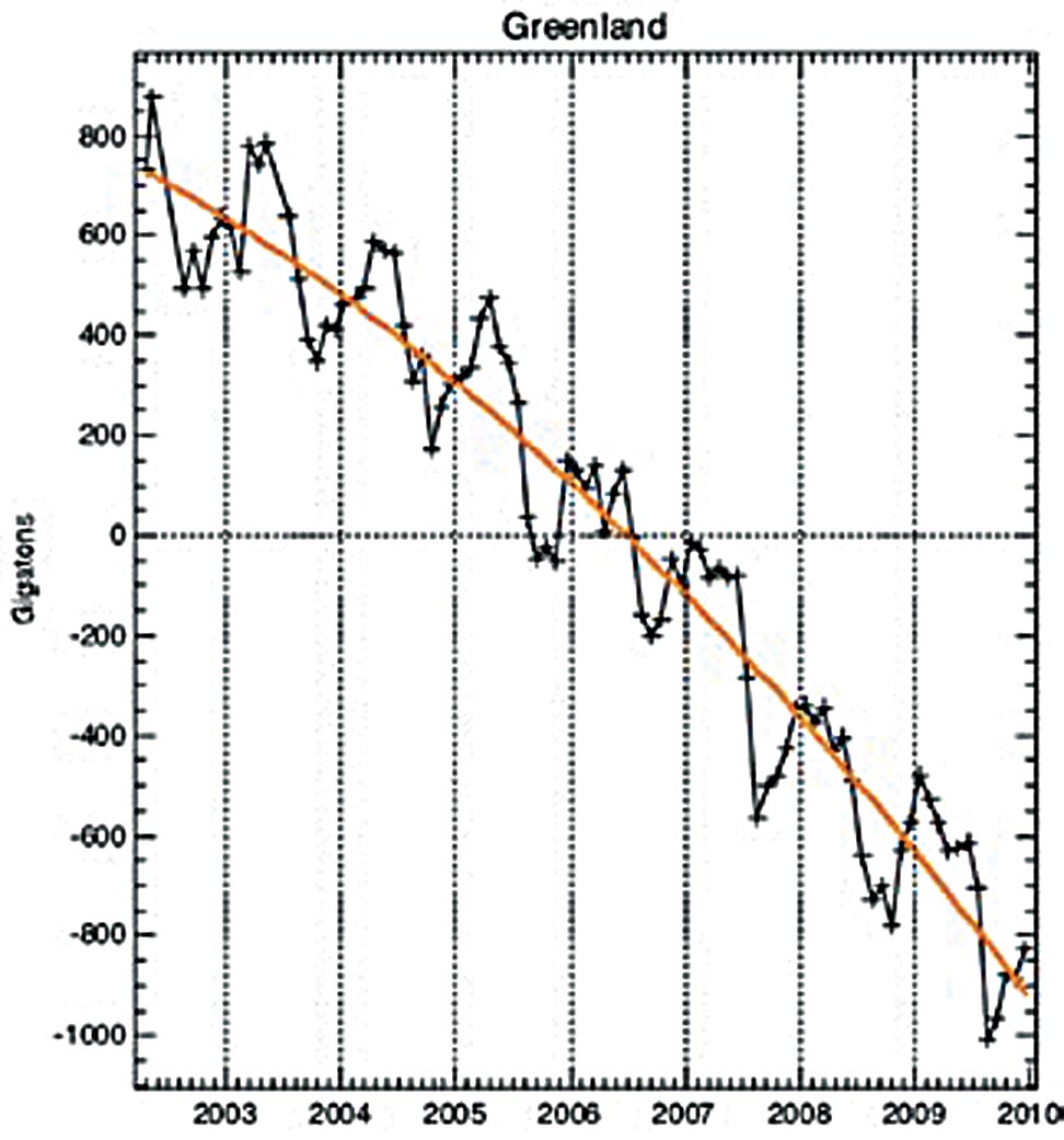
Figure 2. Mass variability summed over the entire Greenland ice sheet, between April 2002 and December 2009. The black line depicts monthly Gravity Recovery and Climate Experiment (GRACE) results; the orange line is a smoothed version.
|
As shown in Figure 2, the sheet is melting fastest along the southeastern shore of the island and in a smaller region on the western shore; Figure 3 displays the total mass of the sheet at monthly intervals since 2002. The seasonal variations, a result of the accumulation of snow and ice in winter and the melting thereof in summer, are plainly visible, as is the downward sloping trend line. The fact that the trend line curves downward from left to right leaves little doubt that the ice sheet is disappearing at a steadily increasing rate. Observers on the ground have long suspected as much, but evidence has been hard to come by. At last, their suspicions are confirmed! GRACE data indicates that the Antarctic ice sheet is disappearing as well, but at a more nearly constant rate.
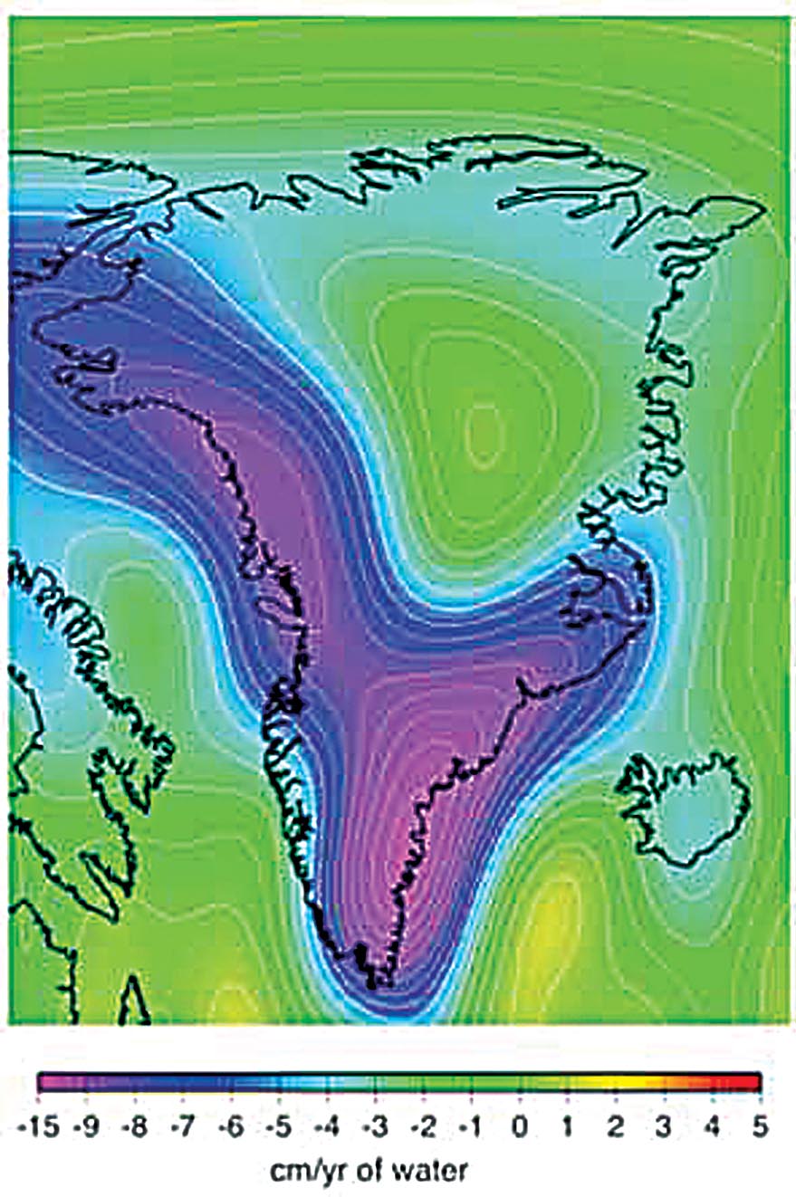
Figure 3. Distribution of mass loss rate across Greenland, as determined from the GRACE solutions.
|
James Case writes from Baltimore, Maryland.